DEVS model of traffic lanes merging

General Information

• The assignment can be made in groups of upto 3 people. It is understood that all partners will understand the complete assignment (and will be able to answer questions about it).
• Grading will be done based on correctness and completeness of the solution. Do not forget to document your requirements, assumptions, design, simulation results, conclusions in detail !

The problem

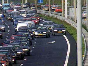
As shown in Figure 1 at a high level of abstraction, two lanes (A and B) join into a single lane.

For each lane, considered of a certain length, the car inter-arrival time is sampled from a uniform distribution. The leftmost blocks denote car arrival (similar to a GPSS GENERATE block).

The two lanes act as infinite capacity carriers of cars: when a car arrives on a lane, it queues in that lane (in order of arrival) until it can enter the junction road segment. The physical position of cars is not considered, only their ordering.

If the junction is free and only one of the lanes has at least one car in it (lane A for example), then the car at the head of lane A can go right through. Actually, to make the model more realistic, we introduce some time delays:

• before the car enters the junction, the driver spends a small amount of time e to make sure the other lane as well as the junction are clear.
• the junction road segment acts as a delay: when a car is in the junction, it remains there for a period of time K (derived from the road segment's length and the car's velocity), during which other cars cannot enter the junction.

If the junction is free and both lanes have at least one car in them, we must decide on a strategy to select a car to enter the junction. You will experiment with two strategies.

1. ``Survival of the fittest'' strategy

Each car (its driver, actually) is assigned, upon creation, an ``aggressiveness factor''. This factor is an integer between 1 and 10, inclusive. The higher the number, the more aggresive the driver. If there is a car at the head of both lanes, the one with the highest aggressiveness factor go through the junction. In case of a tie, one is chosen randomly.

Before the car enters the junction, the driver needs to spend a small amount of time to check that the other lane is not empty, to make eye contact with the other driver, and to intimidate him/her into letting himself/herself pass. The smaller the difference between the aggressiveness factors of both drivers, the longer the intimidation time t_i is. We will use the formula

ti =  a 1+|Af - Bf| ,

where a is some parameter, A_f and B_f are the respective aggressiveness factors.

2. ``Zipper'' strategy

In this strategy, cars from either lane alternate strictly. Each driver always lets at most one car from the other lane go first such that there is strict alternation. Waiting to let a car from the other lane go first is of course only done if both lanes have a car in them. As no time is spent on intimidation in this strategy, drivers only spend the regular time e checking the other lane and the junction before entering the junction.

With both strategies, recall that a car remains in the junction for a time K.

Performance analysis

The transit time of a car is the time between its creation and its departure from the junction.

The average transit time is computed for a sufficiently high number of cars going through the junction.

You will compute the performance metric average transit time for various traffic loads for both scenarios.

In all cases, e = 0.1 s, K = 5.0 s, a = 6

Uniform distributions of Inter-arrival times for cars on both lanes are uniformly distributed in [m-1, m+1] with m varying from 1.5 to 30.

Plot average transit time as a function of mean inter-arrival time for both scenarios and draw conclusions.

Hints and suggestions

• Start by writing the Car class, which contains an attribute for the aggressiveness factor, and another one to remember the time when the car was created.
• You will need four types of atomic-DEVS, which will be combined into a coupled-DEVS:

  1. Generator: generate Car objects according to a uniform distribution. To properly initialize the car's creation time attribute, the Generator must know the global simulation time.
  2. Queue: an unbounded queue of Car objects. The queue receives cars from a generator. Whenever the queue is not empty, it communicates with the junction DEVS to know when it can send a car.
  3. Junction: Can receive a Car object from either lane (Queue submodel), and hold it for a period of time K. Since this DEVS is likely to be interrupted by either Queue while it is busy with a car, it must remember the ``time spent so far on a car'' ! This is where the alternative strategies are implemented. It is a good idea to use inheritance to define specialized methods.
  4. Statistics: receive Car objects from the Junction, and updates the average transit time. Optionally, you would also compute standard deviation to get insight into how peaked the distribution is. To properly compute the transit time of a car, this DEVS must also know the global simulation time.
• Termination condition: the simple DEVS simulator you are working with has but a single termination condition. The method Simulator.simulate takes as a single parameter the length of the simulation.

  We would like to change that condition so that the simulation terminates when a specified number of cars have passed the junction. For this you will need to modify slightly the method Simulator.simulate. It is easy to do if your Statistics DEVS has an attribute that counts the cars as they pass: if this attribute is called X, it can be checked from the method with self.model.statDEVS.X, where statDEVS is the coupled-DEVS attribute to which the Statistics DEVS instance is assigned.

• If you write a script where several simulation runs are performed, it is preferable to re-instantiate both the coupled-DEVS and the Simulator class before each run.

Practical issues

You will use the PythonDEVS simulator found on the MSDL DEVS page.

You need DEVS.py and Simulator.py. template.py is a meaninful starting point. Queue.py demonstrates how to model a cascade of processors (of jobs) in PythonDEVS. An outdated version of this example is given in a report. This report gives background information on the implementation of the DEVS simulator.