|
[PDF version of this document]
Requirements for the assignment are described on the assignment web page. The whole solution can be downloaded here (just untar in ATOM3.asgn).
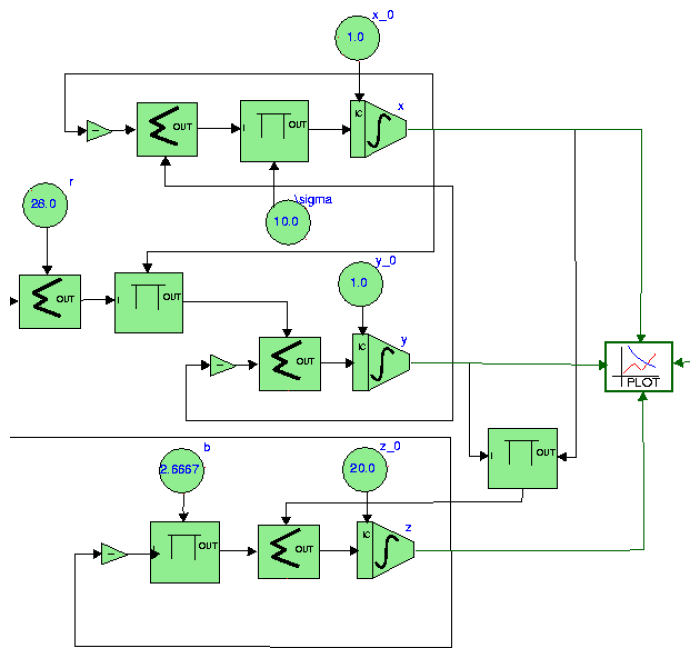
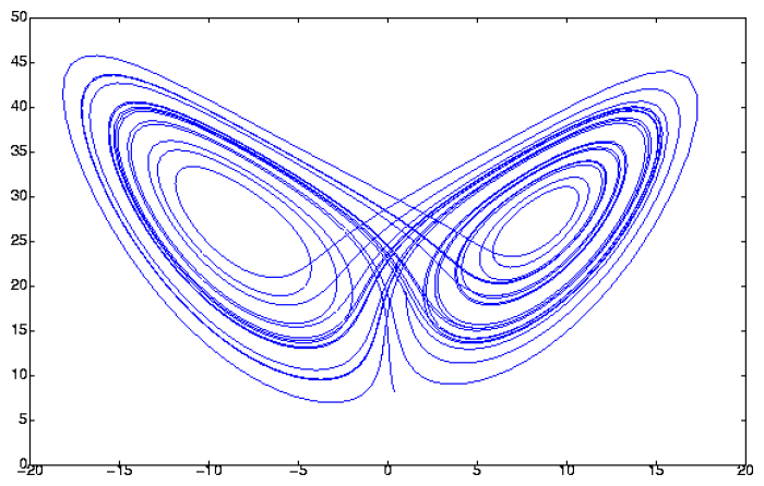
The circle test model is given with the assignment. As required, we built a CBD for the ballistic problem. We also built a CBD for the Lorenz equations (not required - for testing purposes).
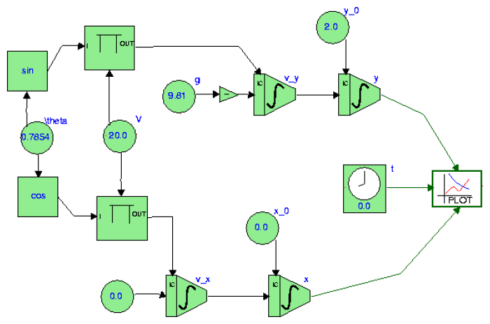
Our CBD for the ballistic problem can be found
here. Whether or not this model
can be simulated by your Time-Slicing simulator depends on how your simulator
processes Generic blocks. The angle (block marked
theta) is in radians.
|
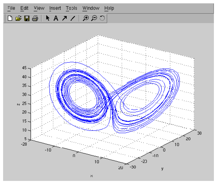
We also developped a CBD for the Lorenz Equations (this was not required). The model can be found here.
|
Algorithms to export to LATEX or to a MatLab (or Octave) m-file are very similar: both files EXPORT_LaTeX.py and EXPORT_Mfile.py import the module Traversal.py.
In Traversal.py are 2 functions that allow to traverse the graph backward from a given connector, building a string summary of the traversal on the way. A boolean flag in those functions specifies which format we are interested in (LATEX or m-file).
A few remarks on the exporting algorithms:
The function EXPORT_LaTeX.exportLaTeX identifies all integrator blocks in the model. For each of these blocks, it calls Traversal.traverse on the input connector to build the ODE, and on the IC connector to build the initial conditions. In this case, Traversal.traverse's recursion stops when either:
Exporting the ballistic model generates the file
\documentclass[12pt]{article}
\begin{document}

\[
  \left\{
    \begin{array}{ll}
      \dot{v_x} = 0.0, & v_x(t_0) = v_{x,0}\\
      \dot{v_y} = -(g) , & v_y(t_0) = v_{y,0}\\
      \dot{x} = v_x, & x(t_0) = x_0\\
      \dot{y} = v_y, & y(t_0) = y_0\\
      \\
      v_{x,0} = cos(\theta)\cdot V\\
      \theta = 0.7854\\
      V = 20.0\\
      g = 9.81\\
      v_{y,0} = V\cdot sin(\theta)\\
      x_0 = 0.0\\
      y_0 = 2.0\\
    \end{array}
  \right.
\]

\end{document}
This gives:
|
Even though the CBD for the model does not show it, the two product blocks have a name. Removing these names in the model will have an impact on its ``denotational semantics''.
As in the previous case, the function EXPORT_Mfile.exportMfile identifies all integrator blocks in the model, and calls Traversal.traverse on the input connector to build the ODE, and on the IC connector to build the initial conditions. Traversal.traverse's recursion stops when either:
To each integrator block must be assigned a unique integer that will be used as a vector index in MatLab. The dictionnary lookUp maps the integrator names to the corresponding indexes.
Note that the ODE solvers are different in MatLab and Octave. The m-file
generated by our algorithm is to be used with MatLab. In MatLab, the function
for the ODE itself must be in a dedicated file. The initial conditions and
the initial/final times are passed as parameters to the ODE solver itself.
Hence the file we produce cannot be used as it is by MatLab. We leave it as it
is, because we don't want to create 2 separate files. The initial condition
x0 included in the generated file must be passed as a parameter to the
ODE solver. In MatLab, the syntax is:
>> [t x] = ode45('filename', [t_init t_final
],x0);
where filename is the name of the m-file. Note that the name of the
function is the same as the filename (minus extension and path). For instance,
generating an m-file for the ballistic problem and saving it under
ballistic.m, we will have:
function xdot = ballistic(t, x)
xdot = zeros(4, 1);
xdot(1) = 0.0;
xdot(2) = -(9.81) ;
xdot(3) = x(1);
xdot(4) = x(2);

x0 = [cos(0.7854)*20.0; 20.0*sin(0.7854); 0.0; 2.0];
|
|
|
Pseudo-code for the time-slicing simulator was given here. Relevant files are:
The current version of the Time-Slicing simulator has some limitations:
The file Graph.py implements both the topSort (topological sorting) and strongComp (identification of strongly coupled components) functions.
topSort takes as an input the list of all Block connectors, and returns the same list sorted in topological order (the sorted dependency graph). A few things to note:
strongComp takes as an input the sorted dependency graph obtained through topSort and returns a list of lists, each sublist a set of strongly connected components. Iff the length of every sublists is 1, then there are no strongly coupled components.
The Time-Slicing simulator in implemented in the file SIM_startResume.py+, in the class TS_Simulator (replacing the class Generator of the original code). Note that this class is implemented twice: see below for explanations (only look at the first implementation for now).
The algorithm follows closely the pseudo-code. To support the PAUSE and RESUME features of the AToM3 environment, the simulator itself is split into two methods:
|
We note that algebraic blocks must be processed in different ways:
The control of the simulation from the AToM3 environment, through the START/RESUME, PAUSE and RESET buttons, works OK. For this, we needed to modify class SIM_startResume.SimulatorThread (replacing the class GeneratorThread of the original code), and the event function SIM_startResume.startResume. Files SIM_reset.py and SIM_pause.py needed to be modified as well, but MODEL_plotWindow.py was left untouched.
It is possible that some AToM3 operations result in unexpected behaviours (e.g., switching models or modifying a model during a session, leaving AToM3 during a simulation, playing too much with the plot window...)
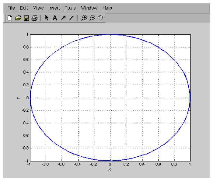
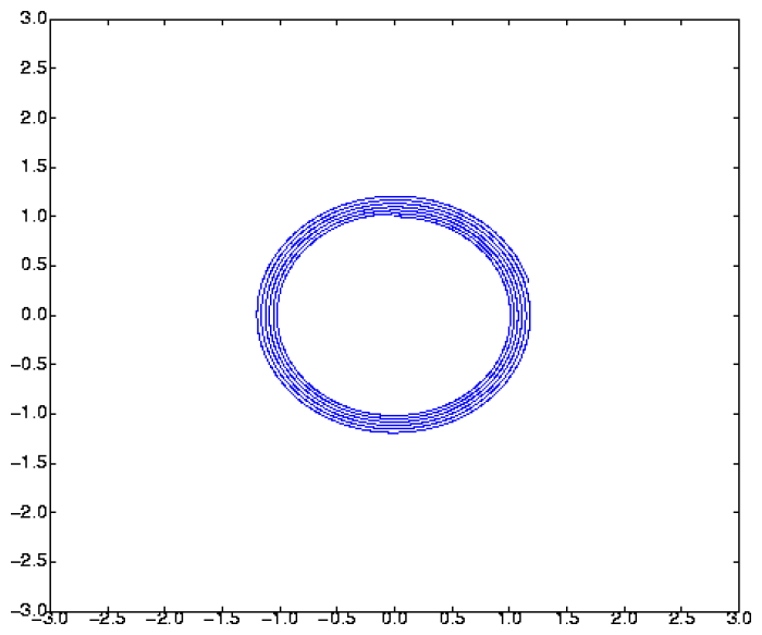
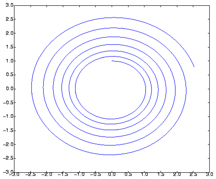
For the circle test problem, the analytical solution should look as a circle in phase space. However, since we use a simple Euler-Cauchy (first-order) approximation we expect that our numerical solution in phase space will look more like a spiral. The bigger the time-step, the more dramatic the effect. The following figures confirm this (compare with Figure 3, which was obtained with Runge-Kutta-Fehlberg - fourth order with embedded fifth order):
|
|
|
|
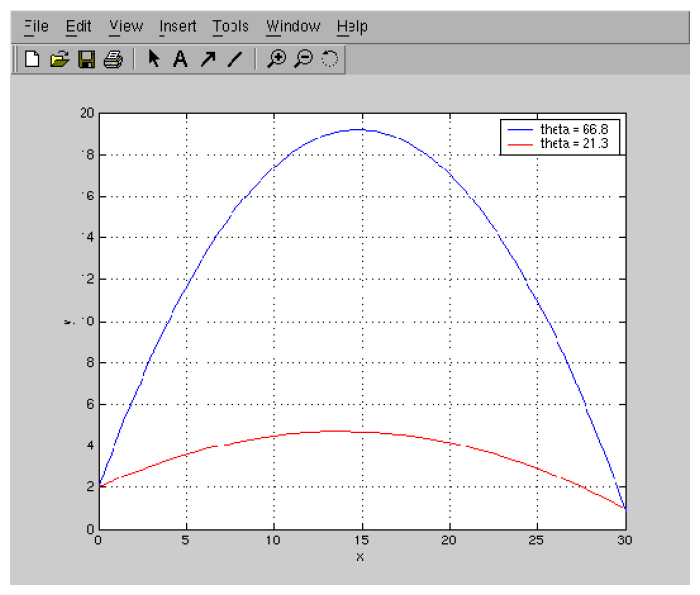
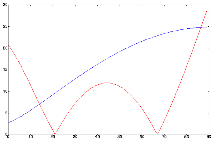
To find the optimal solution for the ballistic problem, we hacked the file SIM_startResume.py: the second definition of class TS_Simulator is solely dedicated to solve this problem (we actually pasted and modified the whole original class - this is not elegant, but faster...). It does several simulations of the ballistic problem, with the initial angle varying between 0.0° and 90.0°. The simulation now terminates when the height of the projectile reaches 1. After each simulation we plot, with respect to the angle, both the length of the simulation and the absolute difference between the projectile distance and its target distance (i.e., 30.0).
Results are shown below: the horizontal axis is the angle (in degrees). In blue, the duration of the simulation (multiplied by 6). In red, the absolute difference between projectile distance and target distance.
|
We see the target is reached when the angle is approximately 22°, and 67°. But the time to reach the target is much smaller in the first case. This is the solution we were looking for!
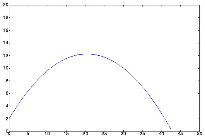
The analytical solution for the ballistic problem can be found to be:
|
|