• The due date is Wednesday 8 December 2013, before 23:55.
  
  
• Submissions must be done via BlackBoard. Beware that BlackBoard's clock may differ slightly from yours. All results must be uploaded to BlackBoard and accessible from links in the main (index.html) file. There is no need to upload AToM³.
  
  
• The assignment must be made in groups of maximum 2 people. It is understood that all partners will understand the complete assignment (and will be able to answer questions about it). Clearly identify who did what.
  
  
• Grading will be done based on correctness and completeness of the solution. Do not forget to document your requirements, assumptions, design, implementation and modelling and simulation results in detail!
  
  

This assignment will make you familiar with Statechart modelling, simulation, and code synthesis (and a bit of testing).

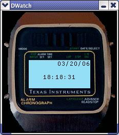
In this assignment, you will design a Statechart model specifying the reactive behaviour of a Digital Watch (inspired by the 1981 Texas Instruments LCD Alarm Chronograph).

You will first model the reactive behaviour of the watch in the DCharts formalism (a variant of Statecharts) in the tool AToM³.

The Statechart simulator SVM (as a plugin of AToM³) will allow you to check, by means of simulation, whether your model behaves according to the requirements.

Note that it is good practice to start modelling and trying out (after simulation and subsequently, code synthesis) small parts of the desired behaviour in isolation. These can be saved and later loaded to build the full solution Statechart.

The model (saved as DigitalWatchStatechart_DCharts_MDL.py) and its visual representation must both be included in your index.html solution page. The visual representation is obtained by printing the model to file in Postscript format from AToM³ as DigitalWatchStatechart_DCharts_MDL.eps and subsequently converting it to a bitmap (e.g., DigitalWatchStatechart_DCharts_MDL.gif). Alternately, you can print the model to file in SVG (Scalable Vector Graphics) format as DigitalWatchStatechart_DCharts_MDL.svg and include it as such in your solution (as browsers such as Firefox now support SVG).

The application's reactive behaviour (Python code) will be synthesized from the Statechart.

The software application (DigitalWatch.py) is composed of a static component, a controller, and a dynamic component.

The static component (DigitalWatchGUI.py) implements the visual aspects of the watch such as buttons, the display and the Indiglo light and organizes them into a graphical user interface (built using Tkinter, the standard Python interface to the Tk GUI toolkit).

The dynamic component (DigitalWatchStatechart_DCharts_MDL_Compiled.py) will be automatically generated from your Statecharts model. This is done by pressing the "Generate .des" button in AToM³, saving your model as a .des file, and continuing to compilation with the default parameters -l tkinter.

The communication between the static and the dynamic components is handled by the controller (found in DigitalWatchGUI.py). User events such as button press/release are passed from the GUI to the Statechart (as strings) by the controller. Conversely, the Statechart modifies the (visual) state of the GUI by invoking the controller's methods.

Note that the Statechart receives a reference to the controller object as a parameter of the start event when, at application startup time, it goes from its initial state Setup to the state Running.

1. [5%] The time value should be updated every second, even when it is not displayed (as for example, when the chrono is running). However, time is not updated when it is being edited.
2. [10%] Pressing the top right button turns on the Indiglo light. The light stays on for as long as the button remains pressed. From the moment the button is released, the light stays on for 2 more seconds, after which it is turned off.
3. [5%] Pressing the top left button alternates between the chrono and the time display modes. The system starts in the time display mode. In this mode, the time (HH:MM:SS) and date (MM/DD/YY) are displayed.
4. [20%] When in chrono display mode, the elapsed time is displayed MM:SS:FF (with FF hundreths of a second). Initially, the chrono starts at 00:00:00. The bottom right button is used to start the chrono. The running chrono updates in 1/100 second increments. Subsequently pressing the bottom right button will pause/resume the chrono. Pressing the bottom left button resets the chrono to 00:00:00. The chrono will keep running (when in running mode) or keep its value (when in paused mode), even when the watch is in a different display mode (for example, when the time is displayed).
   Note: interactive simulation (in AToM³) of a model containing time increments of 1/100 second is possible, but it is difficult to manually insert other events. Hence, while you are simulating your model, it is advisable to use larger increments (such as 1/4 second) for simulation purposes.
5. [10%] When in time display mode, the watch will go into time editing mode when the bottom right button is held pressed for at least 1.5 seconds.
6. [20%] When in time display mode, the alarm can be displayed and toggled between on or off by pressing the bottom left button. If the bottom left button is held for 1.5 seconds or more, the watch goes into alarm editing mode. This is not an example of good User Interface design, as going to editing mode will also toggle on/off and that may not be desired. It is however how the 1981 Texas Instruments LCD Alarm Chronograph works. The first time alarm editing mode is entered, the alarm time is set to 12:00:00. The alarm is activated when the alarm time is equal to the time in display mode. When it is activated, the screen will blink for 4 seconds, then the alarm turns off. Blinking means switching to/from highlighted background (Indiglo) twice per second. The alarm can be turned-off before the elapsed 4 seconds by a user interrupt (i.e.: if any button is pressed). After the alarm is turned off, activity continues exactly where it was left-off. Note that after the alarm finishes (flashing ends), the alarm is un-set (so it will not go off the next day at the same time).
7. [20%] When in (either time or alarm) editing mode, briefly pressing the bottom left button will increase the current selection. Note that it is only possible to increase the current selection, there is no way to decrease or reset the current selection. If the bottom left button is held down, the current selection is incremented automatically every 0.3 seconds. Editing mode should be exited if no editing event occurs for 5 seconds. Holding the bottom right button down for 2 seconds will also exit the editing mode. Pressing the bottom right button for less than 2 seconds will move to the next selection (for example, from editing hours to editing minutes).
8. [10%] Not a behaviour requirement, but related to it ...
   You should pick one of the above requirements and build a testing harnass for it which will determine whether your Statechart satisfies the requirement. You do this by adding orthogonal component(s).

To help clarify the requirements, the following contain a working solution (execOnly_32bit.zip and execOnly_64bit.zip). The Statechart model is only present in compiled form however. Note that these may work on your machine. Though Python source code is highly portable, the bytecode is not.

batteryHalf()
  Sets the battery power to half, making the display show only "8"s.

batteryFull()
  Sets the battery power to full, making the display show as usual.

getTime()
  Returns the current clock time.

getAlarm()
  Returns the alarm time set. 

checkTime()
  Checks if the alarm time set is equal to the current
  clock time. If so, it will broadcast the "alarmStart" event  
  to the statechart and return true.  Otherwise, it returns false.
  Note that checkTime() does not care/check whether the alarm
  has been set "on". 

refreshTimeDisplay()

  Redraw the time with the current internal time value.
  The display does not need to be cleaned before calling
  this function. For instance, if the alarm is currently
  displayed, it will be deleted before drawing the time.
      
refreshChronoDisplay

  See refreshTimeDisplay()
  
refreshDateDisplay()

  See refreshTimeDisplay()
  
refreshAlarmDisplay()

  See refreshTimeDisplay()  
    
resetChrono()

  Resets the internal chrono to 00:00:00.
          
startSelection()

  Selects the leftmost digit group currently displayed on the screen.
    
increaseSelection()
  
  Increases the currently selected digit group's value by one.
  
selectNext()
  
  Select the next digit group, looping back to the leftmost digit group when
  the rightmost digit group is currently selected. If the time is currently 
  displayed on the screen, select also the date digits. If the alarm
  is displayed on the screen, don't select the date digits. (to simplify the
  statechart).
  
stopSelection()
                    
increaseTimeByOne()

  Increase the time by one second. Note how minutes, hours, 
  days, month and year will be modified appropriately, if needed
  (for example, when increaseTimeByOne() is called at time
   11:59:59, the new time will be 12:00:00).
    
increaseChronoByOne()

  Increase the chrono by 1/100 second.
    
setIndiglo()

  Turn on the display background light
    
unsetIndiglo()

  Turn off the display background light
    
setAlarm()

  Flag the alarm to be on or off.
  
  
Events sent to the Statechart (as strings):

(due to button press)

- topRightPressed
- topRightReleased
- topLeftPressed
- topLeftReleased
- bottomRightPressed
- bottomRightReleased
- bottomLeftPressed
- bottomLeftReleased

(generated by checkTime() if current time == alarm time)

- alarmStart

The archive wristwatch.zip contains a very simple example to get you started. This starting point Statechart is reproduced here

• DigitalWatch.py: the main wristwatch application. Do not modify ! Start it with python DigitalWatch.py.
• DigitalWatchGUI.py: the "static" part of the application. It contains the specification of both the GUI and the controller. Do not modify !
• watch.gif, watch.jpg, noteSmall.gif: images needed by DigitalWatchGUI.py.
• DigitalWatchStatechart_DCharts_MDL.py: the visual DCharts model describing a very simple behaviour. This model can be opened in AToM³. To allow simulation, some of the actions are written in [DUMP()] outputs.
• TestFramework_MDL.py: an example model of how to use StateCharts to implement test cases.

The Models/DCharts/ folder in the central AToM³ installation contains some small examples demonstrating various features of Statecharts. The Models/DCharts/TrafficLight/ folder contains the small traffic light example (including the use of orthogonal components to model the "environment").

Please hand in any file that you modified. Include links to these files in your index.html. Also, please include your model as an image. DO NOT include files that weren't modified.

It is good practice to model and simulate different parts of the overall solution in isolation (bottom-up design). You can save them in different files and later load them into a combined model.

The scc Statechart compiler tries to produce speed-optimized code. This, at the expense of memory used. When you use too many orthogonal components this will lead to synthesized code which cannot be compiled/run. Hint: for the assignment, a "natural" solution will require 6 orthogonal components.

AToM³ is installed on the lab machines.
You will find some example models in the central Models DCharts directory (Models/DCharts/). This is a good place to find examples of the [AFTER()], [EVENT()], [INSTATE()], etc. macros.
The svm simulator is installed in the External/ directory of the AToM³ central installation. It is available as a plugin from AToM³. If you encounter threading problems, use only the SCC Statechart compiler. The scc StateChart Compiler can be found in svm's installation directory.

There is extensive documentation on SVM and SCC. This is for example where you will find detailed information on macros (including on how to write your own). For those interested in more in-depth information on SVM and SCC, have a look at Thomas Feng's M.Sc. thesis.

It is possible to install AToM³ and SVM/SCC on your own computer. They should run on (variants of) Windows, Linux, and Mac OS X (as long as Python/Tkinter is installed). Note that due to recent problems with Tkinter, there may be problems on Mac OS X. You need to download the latest version of AToM³ from http://atom3.cs.mcgill.ca/. You will need to download svm-0.3beta4-src.zip found on the same site. It contains SVM/SCC. It is best installed in the External/ directory of your central AToM³ installation. Alternately, it may be installed in your User External folder.