Practical Information
- Due Date: 10 November 2023, before 23:59.
- Team Size: 2 (pair design/programming)
As of the 2017-2018 Academic Year, each International student should team up with a "local" student (i.e., whose Bachelor degree was obtained at the University of Antwerp). - Submission Information:
- Only one member of each team submits a full solution.
- This must be a compressed archive (ZIP, RAR, TAR.GZ...) that includes your report and all models, images, code and other sources that you have used to crate your solution.
- The report must be in PDF and must be accompagnied by all images.
- Images that are too large to render on one page of the PDF must still be rendered on the PDF (even though unclear), and the image label should mention the appropriate file included in the submission archive.
- Make sure to mention the names and student IDs of both team members.
- The other team member must submit a single HTML file containing the coordinates of both team members using this template.
- Submission Medium: BlackBoard Ultra. Beware that BlackBoard's clock may differ slightly from yours. If BlackBoard is not reachable due to an (unpredicted) maintenance, you should submit your solution via e-mail to the TA. Make sure all group members are in CC!
- Contact / TA: Rakshit Mittal.
Goals
In this assignment, you will use the Modelica Language to create a simple car cruise controller. You will learn:
- How Ordinary Differential Equations (ODE) can be used for the modeling and simulation of Cyber-Physical Systems (CPS).
- Furthermore, you will learn how a generic model must be calibrated to fit real-world data.
- You will then design and model a controller to control the CPS.
- You will finally tune the control parameters to optimize some goal function based on the (resultant) behavior of the CPS.
- You will devise policy based on the tuned controller. This policy is used to calculate the permissible limits of the set-point of the controller.
OpenModelica
For the tutorial on Friday 27 October, you should make sure you have OMEdit installed in your laptops. You should also have downloaded this zip-file which contains an example model of cooling of an object based on Newton's law of cooling and corresponding Python code.
You will use OpenModelica to perform all the tasks. You can install the latest stable version of OpenModelica on your systems by following the directions by going to the OpenModelica website > Download > Windows/Linux/Mac (based on your OS). Choose the 'Official Release' package.
Installing OpenModelica installs a number of applications in your system:
OMEdit
The OpenModelica Connection Editor (OMEdit) is the standard graphical user interface that is used for graphical Modelica model creation and editing. We will use OMEdit for all the tasks. Launch instructions and other features of OMEdit are available on the OMEdit website. OMEdit has 4 different views but we are only interested in the Modelling and Plotting views. We will primarily use OMEdit to design the model. Information about the other OpenModelica applications are just given for information.
OMNotebook
OMNotebook is a notebook-like tool to learn the usage of OpenModelica and construct more-readable documentation which incorporates code-windows in between text. Think of Jupyter Notebooks.
OMShell
OMShell is an interactive session handler that parses and interprets commands and Modelica expressions for evaluation, simulation, plotting, etc. The session handler also contains simple history facilities, and completion of file names and certain identifiers in commands. We will not use OMShell because we want to learn and visualize graphically the models that we are building. Hence we will only use OMEdit.
We use Python because we can then directly use the data obtained from simulation for analysis through a number of data analysis packages available in Python.
One thing to note is that a Modelica model needs to be compiled only once. Once compiled, the parameters can be changed in subsequent executions/simulation runs without having to compile the model again. This is advantageous since compilation can prove to be a significant overhead if we are optimising for a number of different parameters and ranges (read: the number of simulation runs could go into the thousands or more, as I'm doing in my research, but that is the beauty of it).
Basics
While the Modelica language and its capabilities of object-oriented acausal modeling of the multi-physics have already been described in the lectures, what follows is a 'how-to' to get started building your own Modelica models for the assignment using OMEdit.
On the left of the OMEdit window, is the Libraries pane which displays all the libraries that have been loaded in the current Modelica session. Modelica models are organised in Packages which can contain other packages and Modelica classes.
Create a Modelica Package
Go to File > New > New Modelica Class. In the Create New Modelica Class dialog box, enter a valid package name for example, example_package. In Specialization, select Package. Click OK. You should now see your Modelica package in the Libraries class. You should save it before proceeding further by clicking on the corresponding icon in the menu bar or going to File > Save.
If you have already created and saved a package, you can load it in the current session by goign to File > Open Model/Library Files, and choosing the corresponding file in the browsing window.
Create your first Modelica Model
Right click on your Modelica package in the Libraries window > in the drop-down menu select New Modelica Class. In the create New Modelica Class dialog box, enter a valid class name, for example, example_model. In Specialization, select Model. Make sure that for Insert in class, the textbox specifies the Modelica package within which you want to create your Modelica model. Click OK. You have created your first Modelica model!
You can edit the model from within the package or by opening the model. Ideally you should edit the model directly, since then you can visualize it if in the form of blocks and connectors. You cannot visualise a package sinc eit just contains other modelica classes with no phsyical connections between them. The modelica classes are just organised that way since they may be related. For example, the Modelica package contains sub-packages like Electrical (for electrical components), etc. Modelica classes can extend other Modelica classes, i.e. inherit the declarations from the extended class. They may also simply re-use components defined in other Modelica classes.
Build/Edit your Modelica Model
Double click on the Modelica model you want to edit. This takes you to the Modeling view. In the top right corner of the Modeling view are 3 buttons to toggle between different editing interfaces. The 2nd button is to open the Graphical editor and the 3rd button is to open the textual editor.
The graphical editor can only be used in case the model consists of blocks with causal/acausal connections between them. For the 1st and 2nd tasks, you will not use the graphical editor, since we are just creating a model based on Ordinary Differential Equations which have no graphical concrete syntax (within OpenModelica atleast).
In the text editing pane, you can now define your modelica model in-between the model and its corresponding end declarations. Look at the Modelica By Example website for simple introductory examples of Modelica models based on simple Ordinary DIfferential Equations of physics.
If you are making a component-based model. You can add components to the model by dragging them from the Libraries pane onto the graphical editor. You will be prompted to give the component a unique name. You can draw connections between the interfaces of components by holding the left mouse button while simultaneously moving it from one iterface ot the other. This highly intuitive. You can modify parameters of the components by double-clicking on them, which will open the Element Parameters box.
Simulate your Modelica Model in OMEdit
Once you have defined a complete and correct Modelica model, you can now simulate it. To do so, you should click on the S icon in the menu bar. This opens the Simulation Setup dialog box. You can set simulation paramters in this dialog box.
Make sure that you have verified the simulation start time, stop time, step-size/number of intervals, solver method (DASSL is preferred), and tolerance (the default 1e-6 is good enough, as low as possible is preferred ideally).
You can also set the output format to output the data to a file. However, we do not need to do so, since we will later perform simulations through Python where we will handle the simulation output directly. This is just for visualization and initial validation of the model.
Click OK to begin simulation.
Note: You can also 'check' the model by clicking on the tick-mark icon in the menu bar. The output from this can be observed in the message browser. The message browser will tell you if something is missing in the model, or if there are inconsisencies in the model.
Visualize simulation trace
Clicking OK in the Simulation Setup ideally takes you to the Plotting view. If not, you can go to the plotting view through the corresponding tab in the bottom-right corner.
On the right you will see the variable browser. You can select any variable/s to plot them in the pane and observe their values over the simulation. The values indicated in the variables pane is the value of that variable at the end of the simulation.
Parametrizing simulation quantities in OMEdit
To define a parameter you simply have to use the 'parameter' keyword followed by its unit name and default value in this syntax: parameter <unit> <name>(start = <default value>). If you want to parametrize a quantity which is a parameter of a block in your model. Simply double click on the block in the graphical editor and change the parameter value to the parameter name. This value need not be a numeric quantity but it can be a reference to the name of the parameter within the model, or a function of the parameter as well. Once you hve changed the value in the block, go to the textual editor of your model, and use the same syntax as above to define a parameter. Note that the name of this parameter should correspond to the name of the parameter you have defined in the value of the block. Look at the following image for an example: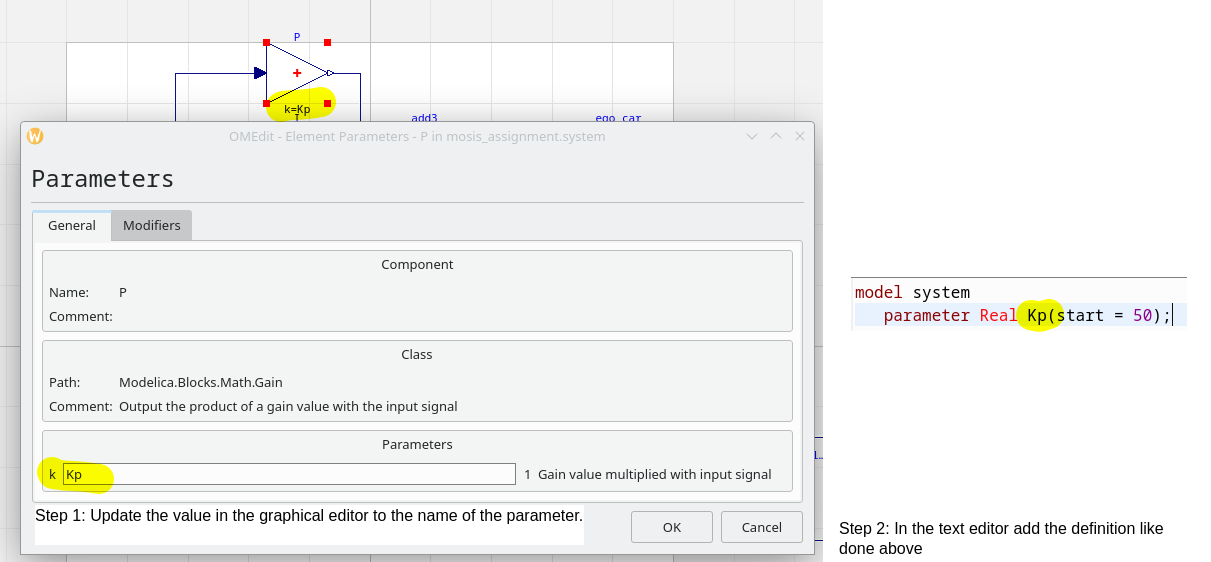
Figure 1: Parametrizing the values of the block-parameters of the blocks in your model.
Multiple simulations and analyses of your Modelica model
The example Python file contained in the zip file describes how to use Python to simulate and visualize data from an example Modelica model which will be introduced in the tutorial as well.
We will perform multiple simulations by generating the executable through OMEdit. You should make sure that the executable is generated and not deleted in the right directory by:
- go to Tools > Options > General > Adjust the value of Working DIrectory as you like. The executable will be stored in selected_working_directory/model_name/ . So, in the example, if I select example as the working directory, the executable will be example/NewtonCooling/NewtonCooling
- go to Tools > Options > General > disable 'Delete entire simulation directory of the model when OMEdit is closed'
To generate these files, once the settings mentioned above are correctly configured, you should simulate the model in OMEdit at least once.
To re-simulate your model, but not from OMEdit you can simply use the terminal command to execute the executable which is in the directory as described above './the_model_name'. For the example, it will be './NewtonCooling'. Note that you should change the current directory of the terminal session to the example/NewtonCooling/ directory before doing so. This cannot be done from within the example/ directory.
The simulation results will be stored in the same directory as the executable. By default it is a MAT-file, and you should try to use the same because it is the most efficient (compared to CSV, etc.). At the end of each simulation you should read the MAT-file, and record the variables that you are interested in before performing the next simulation, because this file will be overwritten during re-simulation. You can read the MAT-files generated by OpenModelica using the readMat function in the example code!
To re-simulate the model, but with different parameters, you can use command line as well. You simply have to structure your command using the -override flag, as the following './model_name -override parameter1=value, parameter2=value ..'. This is also described and demonstrated in the example code.
To implement a loop over the parameter values, you will have to write a Python script. You can execute shell commands using the os package as demonstrated in the example. Take special note that os.changedir function is used to change the working directory of the virtual shell to the results directory.
Assignment Overview
- Plant Model Creation
- Plant Model Calibration
- Controller Model Creation
- Controller Model Tuning
- Policy-Making based on Tuned Controller
Each part is aligned with one of the learning goals
Problem Statement
A cruise-control system is the simplest form of automated driving for automobiles. There are many variations of cruise control systems:
- some which are designed to maintain a constant speed,
- some which are adapted to maintain a constant speed but with awareness of distance to the nearest physical object in front (like a car) to avoid crashing into it,
- or to maintain a constant safe distance to the car in front in cases like vehicular trains / groups / convoys as shown below:

Figure 2: Presidential convoy in the United States.
We will be focusing on the case of a vehicular train / convoy. On highways, it is advantageous for vehicles to move in groups for various reasons. The distance between the vehicles is crucial. If the distance between vehicles is low it is potentially unsafe, while being more efficient in the usage of highway space. However, if the distance is higher, safety is increased but efficiency is decreased.
The control for such a vehicular train can be implemented in many different ways. The simplest case is that each vehicle locally follows the car in front. The more complicated case is when a single platoon-level' algorithm collects information from all vehicles and is able to direct all vehicles simultaneously. We will only model the simple local vehicle control scenario.
Plant Model Creation
We know that the control input to the car, from the controller, is some sort of acceleration-related signal. We will only consider the drag resistance of the car. The drag resistance force acts in the direction opposite to the movement of the car and is proportional to the square of the speed of the car. Hence it is $b \cdot v^2(t)$ where b is the drag coefficient.

Figure 3: (a) Block diagram and (b) free body diagram of the car.
Hence, the equation of the motion of the car is as follows:
$$M \cdot \dfrac{d v(t)}{dt} = ( A \cdot u(t) ) - ( b \cdot v^2(t) )$$This is derived from Newton’s laws of motion. Forces on the car are simply equated to its motion.
Where M is the total mass of the car, v(t) is its velocity as a function of time, A is the forward gain of the electronic control signal u(t) which has unit Volts. The forward gain A from the control signal is an abstraction of the transformation of the actual value of the control signal to the force generated from that signal by the car engine.
Tasks
You are the engineer and the designer/scientist/client has given you the information above. Your task is to model the plant/car using the information given above, in Modelica. Special care should be taken to parametrize the model correctly. The parameters are A, b, and M.
- Implement the given plant equation(s).
Hint: you can use the der(v) function to represent the time-based derivative of the velocity in Modelica. - Model the car's velocity, displacement, and acceleration as variables. The equations should specify the corresponding dependencies between these variables too. i.e. $\dfrac{d v(t)}{dt} = a(t)$ and $\dfrac{d x(t)}{dt} = v(t)$.
- Include your code in your report. It could even be a screen-grab of the editor window.
- Simulate the model with the following values:
- initial velocity = $108 km/hr$
- initial displacement = $0 m$
- $A = 60 N/V$
- $b = 0.86 kg/m$
- $M = 1500 kg$
- $u(t) = 1 V$ (i.e. a constant value throughout time, even though it is a variable)
- The above values (except for $u(t)$) should be set as default values for the model.
- Simulate this model for $400$ seconds with a step size of $0.1$ seconds and provide three separate plots in yoour report: velocity, acceleration and displacement of the car over time. Discuss the results in your report and describe the motion of the car in simple words.
BEWARE! Often customer requirements we will be in multiple units as is done above (for example metres and kilometres). It is your task to unify and express them all in a single unitary system so that your solution is correct. The recommended way is to use SI units in all cases.
BONUS: for explicitly specifying the units of all the variables and parameters in your Modelica model.
Plant Model Calibration
We have created an abstract model of the car, but how to decide the values of the parameters so that model truly represents reality? This is done through parameter calibration. The idea is that, we try combinations of different parameters, and compare the output of the Modelica model, with data from real-life car data. The parameters, which give the least error between the two datas are said to be the best fit, and are chosen accordingly.
Because we designed the car, we know that $A = 60 N/V$ and $M = 1500 kg$.
We need to estimate the parameter $b$ which is the drag coefficient. The real-life data is provided in the csv. The csv contains values for the displacement of the car. The deceleration experiment, for which the data is given in the csv was conducted with the following initial values:
- initial displacement = $0 m$
- initial velocity = $108 km/hr$
- $u(t) = 0 V$ (no input, we are testing the passive deceleration caused by drag)
- $A$ ($60 N/V$) and $M$ ($1500 kg$) are already known as described before
The data from the deceleration experiment is displayed graphically below:

Figure 4: Deceleration profile.
An exhaustive way of finding optimal parameter values (note that in this case, there is only one parameter) is to loop over possible values for the parameters to find the one that gives the closest match mentioned above. This is known as a parameter sweep.
Tasks
The main purpose of this part is finding the drag coefficient of the car $b$, based on experimental data (i.e., observations/measurements on the real system).
- Use the same model as you have done before but adjust the parameters and initial conditions as required for this task. The purpose of setting the parameters to be the same as that in the stopping experiment, is to create a simulation that matches the experiment, except the parameter $b$.
- You need to create a Python script that compiles the Modelica model. The Python file should be named 'parameter_tuning.py'
- This Python script should also contain a loop that iterates over all possible values of $b$ from (0.00 to 3.00]. That means you will have to automatically conduct 300 simulations.
- The Python script should be able to record the trace of the displacement of the car from all of these different simulations. The Python script may store the trace (for each simulation) in memory or save the data as files. You can choose as you prefer.
- Compute the sum of squared errors between each of your experiments/simualtions and the given trace. The simulation that has the smallest total error is the simulation that has the most accurate value for $b$.
- You may compute this directly from the parameter sweep script, but this will be generally slower.
- You are free to chose how you compute this; whether you use Python, Matlab, Excel...
- $b$ will be an integer value with 2 decimal digits in the range (0.00, 3.00].
- Include the plot of error as a function of $b$ in your report. Indicate the value of $b$ for which the error is lowest. Also include a plot of the resulting curve (from your selection of the value of $b$) superimposed with the csv dot plot.
BEWARE! The csv data is at a time-step of 1 seconds, with start time at 0 seconds and stop time at 60 seconds.
BONUS: if your Python code does not compile the Modelica model everytime before new parameters should be updated
Controller Model Creation
A PID (Proportional-Integral-Derivative) controller is widely used in practice to drive the output of the plant towards a set-point. This set-point could change in time. We will however, consider the set-point is constant. In our example, the set-point represents the desired inter-vehicular distance in our convoy. The control output from the PID controller, i.e. $u(t)$ drives the plant / process. The plant produces an output i.e. $y(t)$. The difference between the measured output $y(t)$ and the desired output $r(t)$ (a.k.a the set-point) is called the error $e(t)$. This error value is processed in the PID controller in three different ways as shown in the figure:

Figure 5: PID controller (from Wikipedia).
- Proportional. The error is multiplied by a constant gain $K_p$.
- Integral. The integral of the error (over time) is multiplied by a constant gain $K_i$.
- Derivative. The derivative of the error (over time) is multiplied by a constant gain $K_d$
Hence, the output from the PID controller $u(t)$ is given by:
$$u(t) = (K_p \cdot e(t)) + (K_i \cdot \int_0^t e(t) dt) + (K_d \cdot \dfrac{d e(t)}{dt}) $$The gains $K_p$, $K_i$, and $K_d$ modulate the behavior of the PID controller. You may read more about a PID controller online. The essential point is that three signals are summed, which forms the PID control output $u(t)$. We will also be exploring how the three quantities affect the behavior of the PID control through the tasks.
So, to sum up, in our case:
- The plant is the car.
- The measured output is the measured distance to the car in front.
- The set-point is the desired value of the distance to the front car.
- The control output is an electronic acceleration / deceleration signal to the car.
- The error signal can be the difference of accelerations between the cars, the difference of velocities between the cars, or the difference of distance between the cars. Since in our scenario, we want to maintain a constant intervehicular distance between the vehicles, the error signal is the difference of the distance. One of the tasks is for students to explain and justify this choice further.
Hence the equations for implementing the control are:
$$ e(t) = ( x_l(t) - x(t) ) - r(t) $$where $x_l(t)$ is the position of the lead car and $r(t)$ is constant in time not a variable. $r(t)$ is the set-point or the desired distance between the two cars. $x(t)$ is the position of the ego car, the car which we are interested in controlling, which is following the lead car.
Tasks
You modeled equations using a textual language in the first task. In this task, you will model equations using block diagram representations in Modelica.
Sub-task 1: Setting up
- For this, and the following parts of the assignment, you will use a model of the ego car available here.
- You should do this part and the following parts of the assignment in a new Modelica model. It should be part of the same package as you have used for theprevious tasks.
- Download the provided package on your PC and load it in your OMEdit instance. This package contains the model of the ego car.
- In the graphical editor of your model, add the provided ego_car model as a block.
- The input to this ego_car is the control signal $u(t)$ and the output from the ego_car is its position. The ego_car has parameters initial velocity and initial position. For this task, the initial values are already set to 0. You do not need to change them.Note that input is in Volt and output is in metres.
Imagine that you are an engineer who has been contacted by a company to design a controller for a car that they have developed. They have provided you a model of the car and the cruise-control use-case that they want you to design the controller for.
Sub-task 2: Modelling the scenario/environment by modelling the lead car
- We will represent the motion of the lead car by implementing a look-up table. The look-up table will supply values during the simulation by reading them from data provided by us. The corresponding component is Modelica.Blocks.Tables.CombiTable1Ds. Set smoothness to ConstantSegments and Extrapolation to HoldLastPoint. Set the value of table as '[0, 1.75; 20, -0.75; 40, 0.5; 60, -3.25; 70, 0]', which represents the acceleration profile of the lead car in meter per second-squared. This is the cruise control use case.
- You will have to use integrator blocks to derive the distance travelled by the lead car. You will also have to add any constants of integration using a Constant and a Summation block from the Modelica library. Explore the Modelica library to find these blocks. The equation is: $x_l(t) = x_{l0} + v_{l0}\cdot t + \int_0^t \int_0^t a_l(t) dt dt $ where $x_{l0}$ is the initial position of the lead car and $v_{l0}$ is the initial velocity of the lead car. In our use case, the initial velocity of the lead car is 9 km/hr and its initial position is 10 mtrs.
- Note that when you are connecting the look-up table block to the integrator, you will be prompted to "specify the ndexes to connect the connectors". The value should be combiTable1DS.y[1] and not [:] (the default value)
- Also not that that the input to the lookup table is provided from a Modelica.blocks.Sources.ContinuousClock block.
- In our use-case, the desired inter-vehicular distance is 10 mtrs.
- The above should help you model the error signal using blocks available in the Modelica library.
- With the help of the diagram of a PID controller, implement your own PID control loop. Do NOT use pre-defined PID Controller blocks from the Modelica library. Parametrize the 3 control parameters so they can be varied between simulation runs. Include an image of the block diagram in your report.
- Set $K_p=1$, $K_i=1$, $K_d=20$. Report the simulation traces from time = 0 to 70 seconds. Describe the trace and the outcomes in the report.
- Vary $K_p$ only to study its effect on the behavior of the ego car. Do the same individually with the other two parameters. Include these studies in the report.
For more clarity about modeling the error signal, the block diagram of the PID-control loop should be like this:

Figure 6: PID control loop with scenario implemented.
BONUS: If you encapsulate the PID elements in one PID controller block.
BONUS: If you encapsulate the function to derive the displacement of the lead car from the acceleration supplied by the look-up table in one 'lead_car' block.
Examples on how to compose blocks in Modelica is described on this site. These example blocks are available in the Modelica library.
Note: The case study scenario describes an extreme case study. If the controller behaves correctly in the extreme cases, its correct behavior during normal operation is more certain. Imagine the presidential convoy. The ego car is the presidential car which is following the guard car. The presidential car has momentarily stopped and its velocity is zero (maybe in a busy area) while the guard car moves ahead at 9 km/hr (under the speed limit for crowded areas in Belgium). Suddenly a threat is perceived and the convoy should rapidly exit the location. They accelerate at a very high speed for 20 seconds and then slow down to regroup for another 20 seconds. Once the situation is ascertained, the convoy picks up speed during the next 20 seconds to arrive at its destination where it rapidly decelerates to a stop within 10 seconds. The acceleration, velocity, and displacement profiles of the lead car ares displayed graphically below:
Note: Do not model any part of the control loop using textual equations. In this part of the assignment you should use the graphical view to model your equations. Only use the textual syntax to define the parameters of your model.


Figure 7: Acceleration, velocity, and displacement profiles of the lead car in the scenario.
Controller Model Tuning
Similar to the calibration of the plant, the controller also needs to be tuned for the most ideal solution. However, we do not directly have reference data to compare the simulation output to. Instead, the designer (you) should come up with a cost function to ascertain if the plant behaves as required.
Tasks
- What is the desired position of the ego car? The definition relative to the position of the lead car is that it should be 10 mtrs behind the lead car. Hence, the desired position of the presidential car is simply $x_l(t)$ - 10 mtrs. This is the ideal solution to which you will have to compare the output from the simulation. Remember that in this case, the output from the simulation is the position of the ego car.
- Using Python, simulate the entire model of the plant and controller multiple times with varying combinations of control parameters. Let's say that from past experience, you know that the ideal control parameters will fall in the following ranges:
- $200 < K_p < 400$ (only multiples of 10, higher resolution is not required)
- $1 \leq K_i \leq 20$ (only whole numbers, higher resolution is not required)
- $1 \leq K_d \leq 20$ (only whole numbers, higher resolution is not required)
- Find the RMSE between the desired position versus the position of the ego car for all the simulation traces.
- The simulation trace with the lowest errors was produced with the best control parameters. Report the trace of the position of the ego car, the lead car, and the error for the duration of the simulation.
Note: Remember that the simulation stop time is 70 seconds. Choose any appropriate step size.
BEWARE: Make sure that your reported best simulation does not involve collision of the cars.
Policy-Making from Tuned Controller Simulations
Congratulations! You have successfully designed a controller that will keep the president of your country safe! However, as a final task, the presidential security team has also asked you to define the minimum safe intervehicular distance they can keep with the controller that you have designed. An unsafe desired intervehicular distance is a set-point that results in a collision between the lead car and the ego car. This happens when their intervehicular distance becomes zero. This happens because as explained in the lecture, PID controllers suffer from problems of overshoot.
Tasks
The presidential team has asked you to report the minimum safe desired intervehicular distance in metres with resolution of one decimal place.
- We have already designed the controller with a desired distance of 10 mtrs. Which means we can test for lower set-points.
- To do this, you will have to parametrize the set-point so that it can be changed in between simulations.
- You will use Python again to simulate the behavior of the ego_car in the same scenario as used in part 3 and 4 of the assignment.
- Start from a set-point of 9.9 and keep going lower until you can find a simulation trace where the two cars collide with each other. Keep your control parameters the same as designed by you in part 4 of the assignment!
- Report the maximum unsafe and the minimum safe desired intervehicular distance that an ego car with your designed PID controller can have. Also report the corresponding behavior traces to show the point of collision.
Practical Issues
- It is allowed to have unresolved "warnings" in your solution, but be aware they might yield different results on other machines.
- While OpenModelica allows the creation of icons for your models, this is not required, necessary or encouraged for the given assignment.