I give here the essence of physical modelling, from a physicist point of view, and without getting into the modelling formalism details like validation of models, the relation between the experiment and the model, etc. which I guess are explained in the course 308-522A given by Hans Vangheluwe...
Modelling a physical system is to give a description of its structure, that is, to describe the state of the system (physical properties) and the state transition mechanism (physical laws). On the other hand, simulating a physical system is to describe its behaviour when specific inputs are given to the system (like initial conditions, driving forces, etc.) (see [1]).
When doing experimentation on a system, we study its behaviour. We can then try to infer a partial model for the system. Then, using simulation, we can compare with actual experimental data to evaluate the validity of the model.
For example, say we want to build a pool table model. Depending if we're a player or a pool table builder, the objective for the model will be different. The player will care mostly about the trajectory of the balls, so that their composition or their cost won't need to be included. On the other hand, the pool table builder will want to care about those parameters.
A hybrid system is a physical system that we model using continuous components as well as discrete components. For example, a bouncing ball is a hybrid system since the evolution of its state variables (position and speed) vary continuously according to Newton laws when falling, but have a discrete change (speed is reversed) when entering in collision with the ground. Note that the discrete change is due by the way we model the collision (for simplicity); in reality, everything is continuous (more on this later).
To model the continuous components, we use ODE's ( [x\dot] = f(x,t)), DAE's (f( [x\dot], x, t) = 0) or even Partial Differential Equations (PDE's) (I won't talk about these though). To model the discrete components, we use FSA and DEVS (Discrete Events Specification).
Or the question could be stated: why discreteness? Indeed, from a classical mechanical point of view, everything is continuous in nature: for example, the collision of the ball with the ground is not an instantaneous event, but in reality is the continuous deformation of the ball (like a spring) which will have the effect at the end of having inverted its speed. This continuous world is no more true in Quantum Mechanics (even though we still use continuous wave functions to model everything...), but this point is not relevant at our level of modelling since QM is rarely present in engineering situations. So then why do we want to use discrete models?
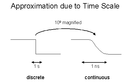
This approximation business is closely related to the time scale we are interested in. For example, if we want to study effects on the ball which occur in a microsecond period, then we'll have to study in details its collision with the ground and not consider it as instantaneous. The time scale gives us approximation thresholds for the problem. Figure 1 shows the effect of the time scale on the continuity of the falling edge of a computer clock signal.
I will briefly mention here that one can want to add the event scheduling formalism to the model. Since I haven't studied this in details yet, I won't say much about it. But one has to be aware that this can be included in Hybrid Systems (and it was included in the simulator described in section 5). Also, for more expressiveness, the FSA can be replaced by DEVS.
So how are the guards implemented? One way to do it in the code
would be to use if-statements:
|
I now give a brief overview of a Hybrid Simulator which was developed by Olivier Dubois and Eric McSween for the course 308-522A in Fall 2001 (see http://www.cs.mcgill.ca/ emcswe/cs522/project/index.html for their web page 1). For the remaining of the presentation, I'll call their simulator the 522 Simulator. This is the simulator I have been using for the past month to study the modelling of Hybrid Systems.
First of all, when we talk about a complete simulator, we're talking about a simulating environment which would need two components: a modelling environment in which we create our models, and simulator kernel which is used to simulate our models. For the 522 Simulator, the simulator kernel was used with a GUI, whereas to create the models, we need to program them in python (using inheritance of some specific classes which provide the modelling environment in some sort).
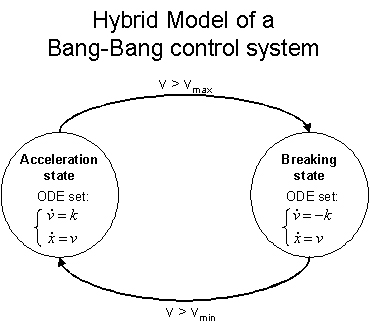
Figure 4 shows a rough (incomplete) UML Class diagram for the 522 Simulator. Three divisions are clearly shown: the simulator kernel, the modelling environment and the model implementation. The details of the simulator kernel are not shown for simplicity. The modelling environment consists of two superclasses: Model (provides the Model interface to the simulator) and FirstOrderDE (which has to be the parent of any specific ODE set). To implement a specific model we need to build a subModel class which will contains the details of the model. If the model contains ODE's, we need to implement those ODE sets by creating a subclass of FirstOrderDE (one subclass of each ODE set). For example, in the Bang-Bang control system example, we could build two subclasses of FirstOrderDE: the BreakingODE and the AccODE which would represent the breaking state ODE and accelerating state ODE respectively.
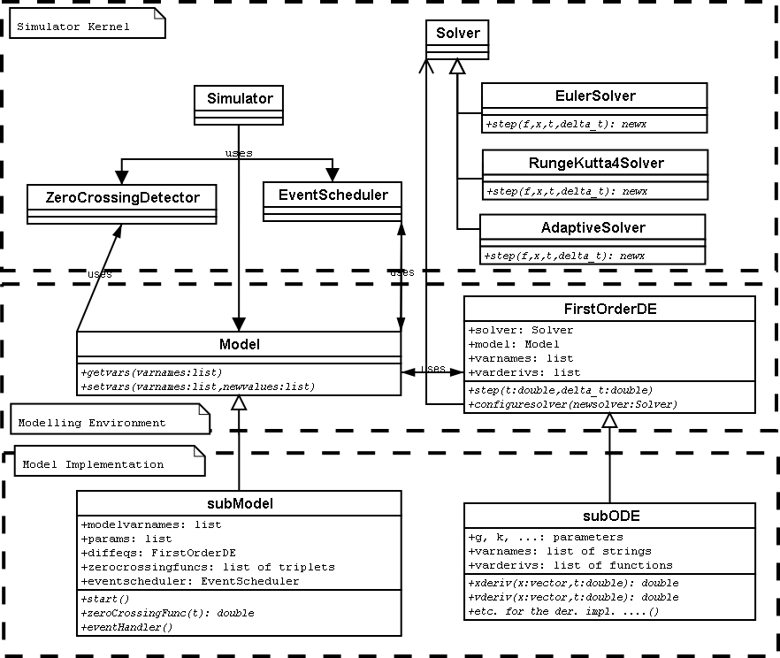
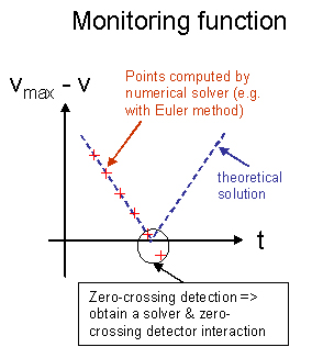
In the subModel class, we need to provide the list of state variables in the model (modelvarnames), a list of the parameters (params), the current state ODE set (in diffeqs), and finally, we need to give a list of triplets for the zerocrossingfuncs variable, which implements the monitoring function mechanism. The triplets contain three things (!): a monitoring function, a condition of crossing which triggers an event (like from positive to negative, negative to positive, or both), and finally an event handler function. So indeed, we need to provide also the monitoring functions definitions and the event handler definitions, which will state what happens what a certain event happens (like changing the current ODE state by changing the diffeqs variable). Finally, we need to provide a start() function which is called by the simulator when the model is initialized.
For the subODE classes, we simply need to provide a derivative function for each of the variables in the ODE set, to represent the [x\dot] = f(x,t) system (where x is a vector). The parameters are also specified (they can then be changed at runtime by the event handlers in the subModel class). A commented example of model implementation of a pool table can be found at http://moncs.cs.mcgill.ca/people/slacoste/research/files/PoolTable.py.
To start the 522 Simulator kernel, we execute the GUI.py file. Figure 5 shows the GUI interface when first starting the simulator. The first thing we need to do is to load a model, by pressing the "click here!" button. I'll load for my first example the module PoolTable.py which contains the subModel and subODE classes for a pool table with a magnetic field model.
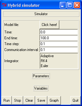
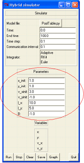
Figure 6 shows the interface after having loaded the model file (PoolTable.py). The first thing we can notice is that the parameters and state variable names are automatically loaded.
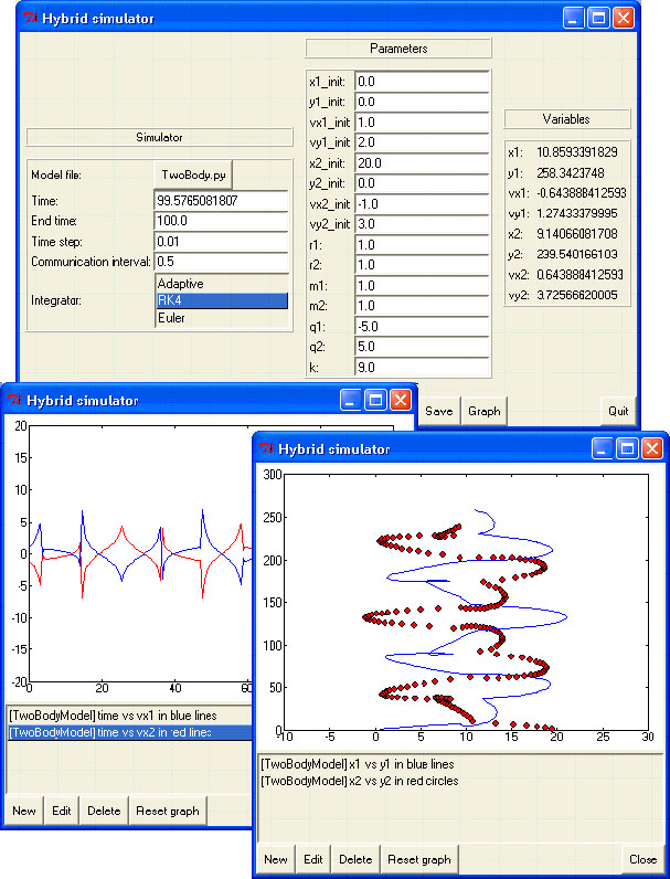
Let me now describe the different fields of the simulator. The "time" field represents the current time of the simulation run (it can be changed to change the starting time of the run). The simulation run is simply started by pressing the "run" button. As the simulation runs, the "time" field and the state variables field are updated to show the evolution of the system. The amount of time before each update of the fields is determined by the "communication interval" field. The "time step" field determines the length of the integration step for the numerical solvers (the smaller the time step, the more precise is the integration). The numerical solver (integrator) can be chosen by clicking the appropriate solver in the ïntegrator" field (Euler is chosen by default).
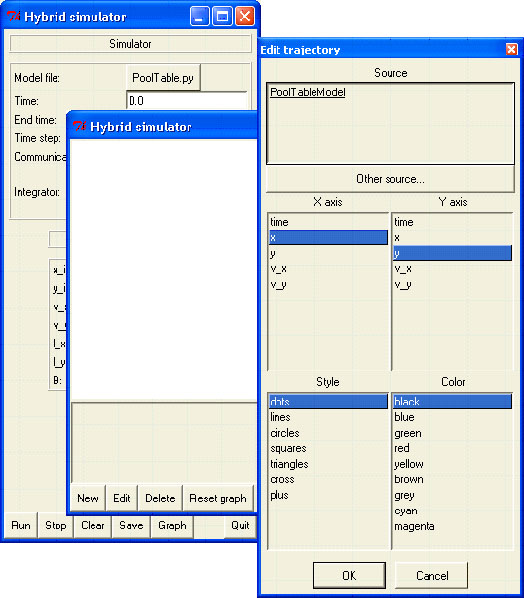
In order to have information about the simulation run, we can create graphs by clicking on the "graph" button (each click creates a new graph). Several trajectories can be added in the same graph by clicking on the "new" button in the appropriate graph. Figure 7 shows the dialog box to edit a trajectory. We decided to graph the y-position of the ball with respect to the x-position, in order to follow the trajectory of the ball. The style for the graph was chosen to be black dots.
When we press the button "run", the simulation starts and the graph is automatically updated (and resized if needed) at the same rate as specified by the communication interval. A sample run for the pool table example is shown in figure 8. Note that we have turned off the magnetic field B (set it to 0) in order to show the periodicity of the problem (and that the collisions with the walls are well detected by the zero-crossing detector). Figure 9 shows another run with a magnetic field of -1.0. A very nice picture! In this case, though, the size of the time step and the numerical solver did make a difference. See the note under the figure for more info.
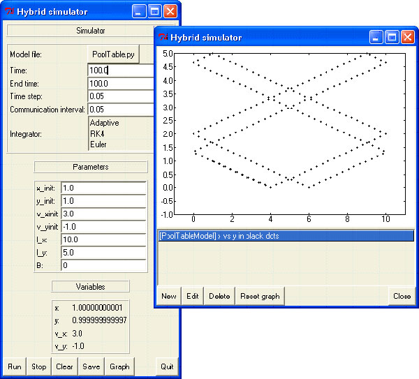
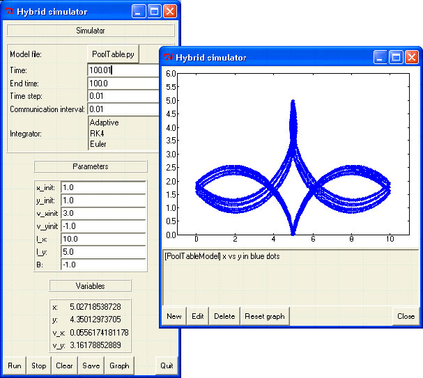
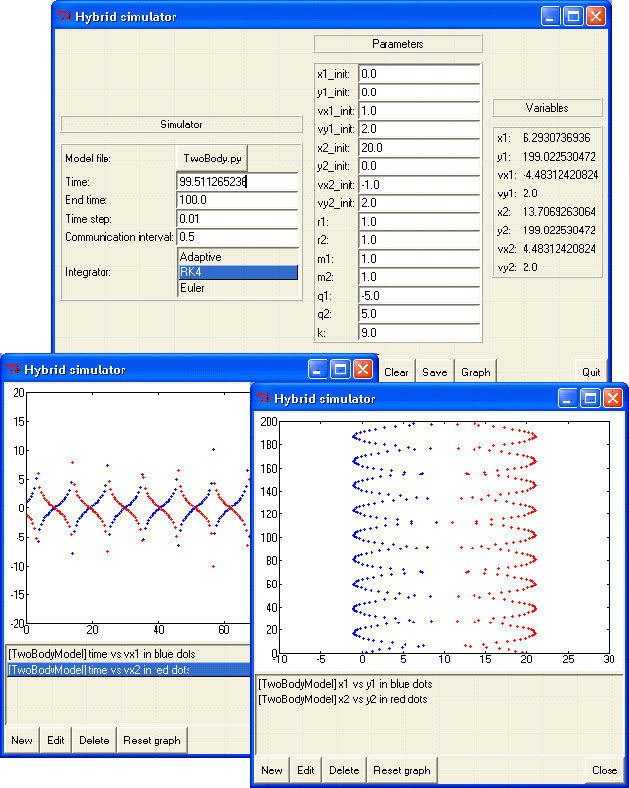
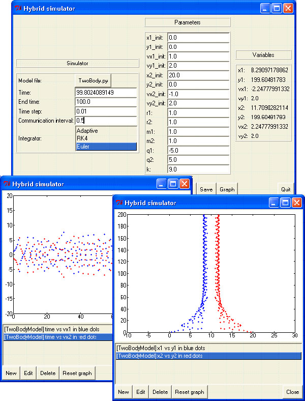
Figure 10 shows a simulation run for a model of two discs with electromagnetic attraction. I have slightly modified the GUI python code in other to make the whole model fits in the screen. The collisions between the discs are assumed to be elastic (these collisions are what make this model hybrid). In this model, r1, m1 and q1 are the radius, the mass and the charge respectively for the first disc. k is the Coulomb's constant. The graph on left of figure 10 shows the horizontal speed of disc 1 (blue) and disc 2 (red) with respect to time. The graph on right shows the trajectory of both discs (using y-position with respect to x-position) (disc 1 in blue, disc 2 in red). The numerical solver was RK4. The symmetry of the trajectory is due to the symmetry of the initial conditions. For comparison between numerical solvers, the exact same problem (same initial condition) but simulated with Euler (with the same time step) is shown in figure 11. We can see a very different trajectory, thus indicating that the solver we use does really matter in our simulation (RK4 is more accurate than Euler).
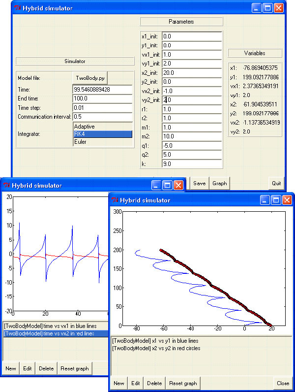
Finally, we can show some other examples. Figure 12 shows the same model but with the mass of disc 2 ten times heavier than the mass of disc 1. The simulation clearly shows the difference (which is due by the conservation of momentum and energy laws). Figure 13 shows a simulation run with a slightly different initial condition for disc 2, thus breaking the symmetry of our problem. The resulting trajectory is a lot more complex, maybe chaotic.
I didn't have any specific goal for this summer; well, at least, not as specific as writing a OCL to python code translator or a UML Class diagram to ER translator...
The most general goal for me was to get a feel for multidisciplinary research and get it touch with a little of many fields about Hybrid Systems, which reunite mathematics, physics and computer science (my three majoring subjects). Since the domain of Hybrid Systems is quite huge, I couldn't do an exhaustive research on the subject (no time, too large). But maybe, by starting with an open mind, we can find something innovative. So in summary, I'll have to trust Hans' experience to orient me in this huge field!
More in relation to the MSDL group, one thing that should be investigated about hybrid systems is to find the best formalism to model them, and the best one to simulate them. The goals for modelling and simulation are different, so we could think to use different formalisms for each and find a way to translate between the two (multi-formalism, this is one of the main components of the MSDL philosophy, right?). The main need for modelling is expressiveness whereas simulation needs efficiency. From a "brief" meeting Hans and I had at the beginning of the summer, one quick hypothesis was to use statecharts for modelling and DEVS for simulation.
Another issue for the modelling vs. simulation part is using causal vs. non-causal modelling. For example, V = RI is a causal form of Ohm's law since if we know R and I, V is known and we don't need to solve for it (R and I are assumed to be the "cause" for V). The non-causal form could be V - RI = 0. There, depending on which variables are known, we are free to solve for the required variable, so no causality has yet been assigned. Explicit ODE's are causal, whereas DAE's are non-causal. ODE's are a lot easier to solve and simulate, but it is a lot easier to model using DAE's directly (since we don't have to solve for the required variable: we can let the computer do it for us, like the Fortran package DASSL (Differential Algebraic System Solver Library) for example). So again, we have here the modelling vs. simulation issue.
Finally, another issue that I'll just mention here is how do we reinitialize state variables after a transition during the simulation. Because the transition of state sometimes changes the whole structure of the equations in our model, we sometimes need to change the value of some state variables in order to obtain physically allowable states which don't violate physical laws (like conservation of energy) for example. How to do this is very far from trivial, and is worth investigating.
The first one would be to study how to improve the 522 Simulator. One improvement could be to add the possibility to use DAE instead of ODE to model, and also to be able to use vectors directly instead of having to use several scalar variables to simulate those vectors. Another improvement would be to re-design the 522 simulator so that it has a modelling component and a simulation component which are more distinct (for now, they are quite intermingled).
Another path (which is quite linked to the first one) would be to add a GUI layer to the modelling environment using AToM3. Using meta-modelling in AToM3, I could specify the syntax of a Hybrid System model, which was roughly described as a FSA with ODE's specified for each state. The user can draw this FSA and type ODE's inside them, etc. in the modelling environment generated by AToM3. Then, using graph grammars, I could generate python code for this model built in AToM3 which could be reused by the 522 simulator.
A third path which is more theoretical and general would be to think about the modularizing and structuring tools for modelling and how to implement them for Hybrid Systems. Those tools come from the object oriented philosophy and some researches have already been done about them in the modelling group in which Hans was a member in Europe, and that I've forgotten the name... The objective is to be able to have maintainability, reusability and generality for our models. Examples of those tools are: using types and classes in our model, using the coupling formalism for the interactions, using inheritance, using multiple levels of abstractions and multiple formalisms. Don't ask me what those are now, I don't know yet! But this could be investigated...
1Note: their class diagram is not
consistent with their final program. You better stick with the
one I have provided in this presentation.