CS-766B Assignment 1
Simon Lacoste-Julien
9921489
February 23 2003
Contents
1 Introduction
2 Part I: Initial Tangent Estimates
2.1 Choosing the kernel
2.2 Normalizing the field
2.3 Plotting the velocity field
2.4 Refinements
2.4.1 Thresholding
2.4.2 Normalization
3 Part II: Co-Circularity Support
3.1 No curvature class
3.2 With Curvature Classes
4 Part III: Relaxation Labelling
5 Conclusion
1 Introduction
I have used the Matlab image processing toolbox to implement this assignment.
There appeared to be quite a lot of technical details to consider
for the implementation, and the experimentation appeared to be quite time
consuming. Several aspects were not mentioned in the article of
Parent and Zucker. I have presented
my answers to each section in a kind of chronological order in order to
see the evolution of my ideas. The images in this report are small and
are only there to give an idea of the results; for better resolution
images, you should consult the electronic version of my report
which is available at
http://moncs.cs.mcgill.ca/MSDL/people/slacoste/school/cs766b/ass1.html.
2 Part I: Initial Tangent Estimates
There were several parameters to estimate in this part and the paper
wasn't very descriptive about how to normalize the tangent estimates
pi(l) so lots of experimentation (trial and error) has
been needed!
2.1 Choosing the kernel
The first step was deciding which parameters to use for the
convolution kernel which acts as a line detector:
|
G(x,y) = Ae-[(y2)/(sy)](e-[(x2)/(s1)]- Be-[(x2)/(s2)] + Ce-[(x2)/(s3)] ) |
| (1) |
I have used as heuristic to first choose s1 to be of the
order of the thickness of the typical vessel we want to detect.
In figure 1, I have shown an example of a typical
vessel that I wanted to detect, with the final kernel chosen
superposed on it. The vessel width was roughly 3 to 4 pixels,
so s1 was chosen to be 2 (since the representative width
of a Gaussian is 2s).
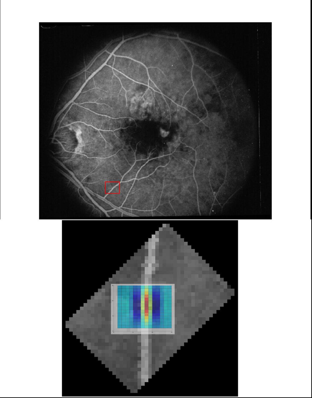 Figure 1: Superposition of kernel over a typical
vessel. The red box shows where the vessel was picked
(it was rotated by 45o for ease of superposition with the kernel).
Figure 1: Superposition of kernel over a typical
vessel. The red box shows where the vessel was picked
(it was rotated by 45o for ease of superposition with the kernel).
The size of the support for the kernel used was taken to be 15×15 like in the article.
The other restriction on the kernel was that its integral in x (sum) should
be 0 so that a uniform background would be killed by it. If this wasn't the
case (say the sum is positive), the regions of the image with a brighter
background would yield noisy lines detection (as I have noticed on my first
trials when the kernel wasn't properly calibrated). This constraint
can be phrased as follows:
|
|
�
x
|
|
�
�
|
y1(x) - B y2(x) + C y3(x) |
�
�
|
= 0 |
| (2) |
where yi(x) = e-x2/si. Assuming one has chosen s2 and
s3, then then this would relate B in function of
the parameter C since the neighborhood is fixed. I have thus plotted several curves in x for the kernel
with different C (see figure 2)
and looked at how they compared with the one in the article to choose a plausible C.
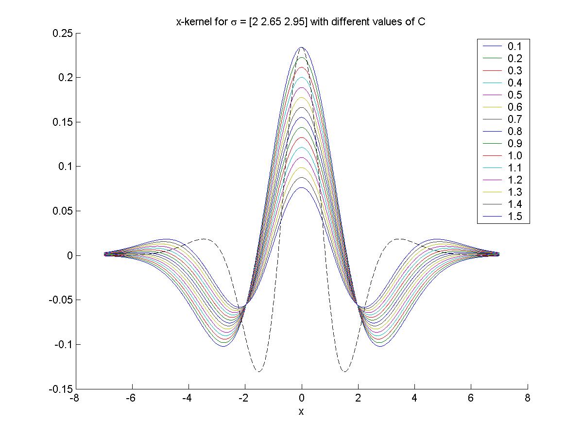 Figure 2: x-kernel variation for different C. The black dotted
line is the x-kernel from the article given in equation (7.1) on p.835.
Figure 2: x-kernel variation for different C. The black dotted
line is the x-kernel from the article given in equation (7.1) on p.835.
I also found that the general shape of the curve wasn't very
sensitive to s2 and s3, which were set to 2.65 and
2.95 respectively. The x-kernel with the final choices of B and C
is shown in figure 3. Notice the difference in width. A summary
of the parameters used is given in table 1, and the 3D shape of
the kernel is given in figure 4.
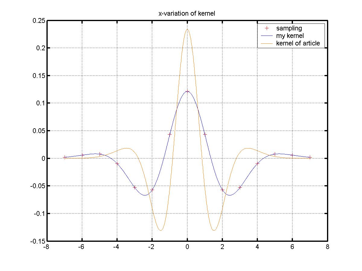 Figure 3: Comparison of my x-kernel with the one of the article.
The parameters used are given in table 1.
Figure 3: Comparison of my x-kernel with the one of the article.
The parameters used are given in table 1.
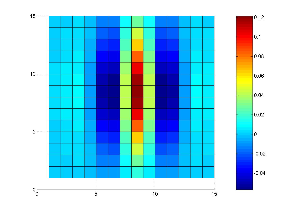 Figure 4: 3D shape of kernel.
| parameter | my kernel | article |
|
|
| s1 | 2.00 | 1.14 |
| s2 | 2.65 | 1.80 |
| s3 | 2.95 | 2.28 |
| sy | 5.00 | 3.60 |
| A | 1 | 1 |
| B | 1.97865 | 1.266 |
| C | 1.1 | 0.5 |
Table 1: Parameters for the kernel
2.2 Normalizing the field
The function filter2 was used in Matlab to convolve the line detector
with the image (in a very efficient way).
In order to apply the line detector at different angles, the
image was rotated using the function imrotate (bicubic interpolation
was used during the rotation). This was simpler to do than rotating the line
detector because of the shape of the neighborhood. 8 orientations were
used (from 0 to 7p/8). After the convolution, we needed to normalize
the values for pi(l) in a proper way. The first way I have used was to
translate the vectors to non-negative values by subtracting the global
minimum (this doesn't change the ordering),
and then scale the values on the interval [0,1] by dividing them
by the global maximum (the images in Matlab need to have intensity values
between in [0,1]) (in matrix operation: P = (P-min(P))/max(P)).
This had the advantage of giving clearer results.
Figure 5 shows a visualization of the resulting tangent estimates
(pi(l)) at 45o. You can truly see that the bright spots coincide
with where vessels were found at 45o.
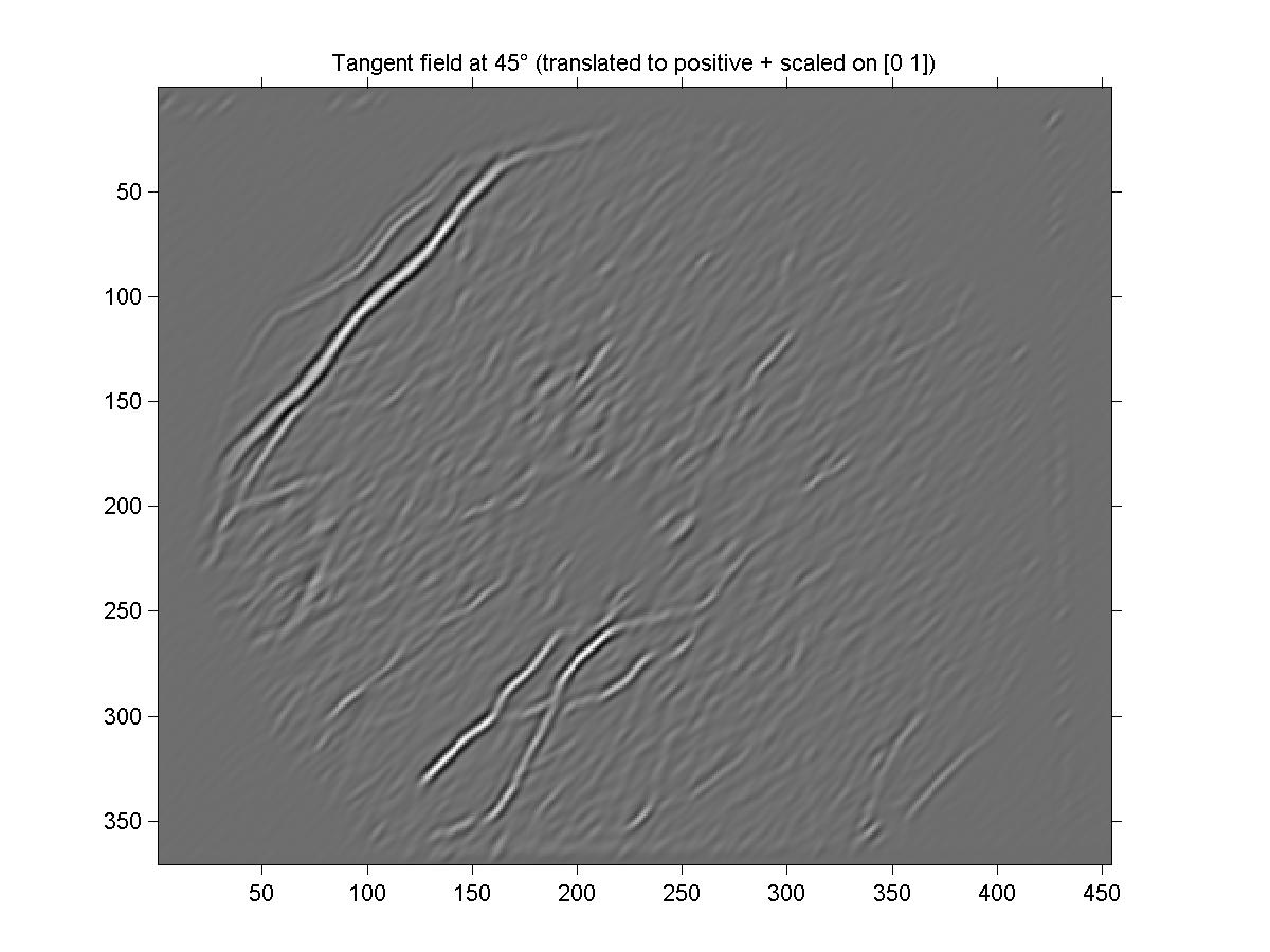 Figure 5: Visualization of tangent confidences at 45o. The function
imshow was used in Matlab to display this image. The uniform grey
background is due to the translation of the values by the global minimum.
The tangent confidences are obtained by convolving the image with our line
detector kernel, and then rescaling the values on [0,1].
Figure 5: Visualization of tangent confidences at 45o. The function
imshow was used in Matlab to display this image. The uniform grey
background is due to the translation of the values by the global minimum.
The tangent confidences are obtained by convolving the image with our line
detector kernel, and then rescaling the values on [0,1].
Other types of normalization will be discussed later.
2.3 Plotting the velocity field
In order to visualize the result in a more global way, the tangent fields were plotted
on the image, with the length of the vectors proportional to their intensity
(using the function quiver). The high density of sampling made
it impossible to see something when a vector was plotted at each pixel, so I have
plotted only the center value of 5×5 blocks (using the function blkproc)
in the image to get an idea of the velocity field. Only tangent estimates greater
than a specific threshold were plotted (again, not to clutter too much the display
and also in order to eliminate the noise from the background). To facilitate the
choice of threshold, I visualized the logical bitmap obtained by the inequality
P > threshold (where P is the matrix of assignments values for a specific l).
For threshold close to the mean, the whole image was mostly white; for meaningful
threshold, only the correct angle lines were kept. The results of this procedure
with my kernel is shown in figure 6. For comparison, the result
with the kernel of the article is shown in figure 7. First of all,
you can see already on these figures that the tangent estimates obtained by
the line detector are already quite good. Also, by comparing the two figures,
you can see that the kernel used in the article was less successful at picking
the vessels with larger width (as expected).
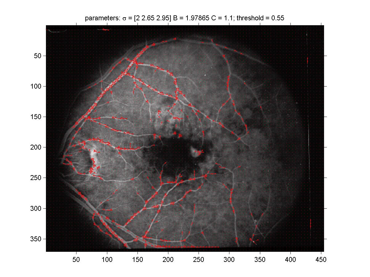 Figure 6: Velocity field arising from my kernel. Note that
the normalization used was translation + uniform scaling (i.e., not
individual rescaling but global rescaling). Center values
of 5×5 blocks is used. Notice that the larger vessels contain
more tangents in this figure than in figure 6, as expected
since the width of the kernel used was bigger.
Figure 6: Velocity field arising from my kernel. Note that
the normalization used was translation + uniform scaling (i.e., not
individual rescaling but global rescaling). Center values
of 5×5 blocks is used. Notice that the larger vessels contain
more tangents in this figure than in figure 6, as expected
since the width of the kernel used was bigger.
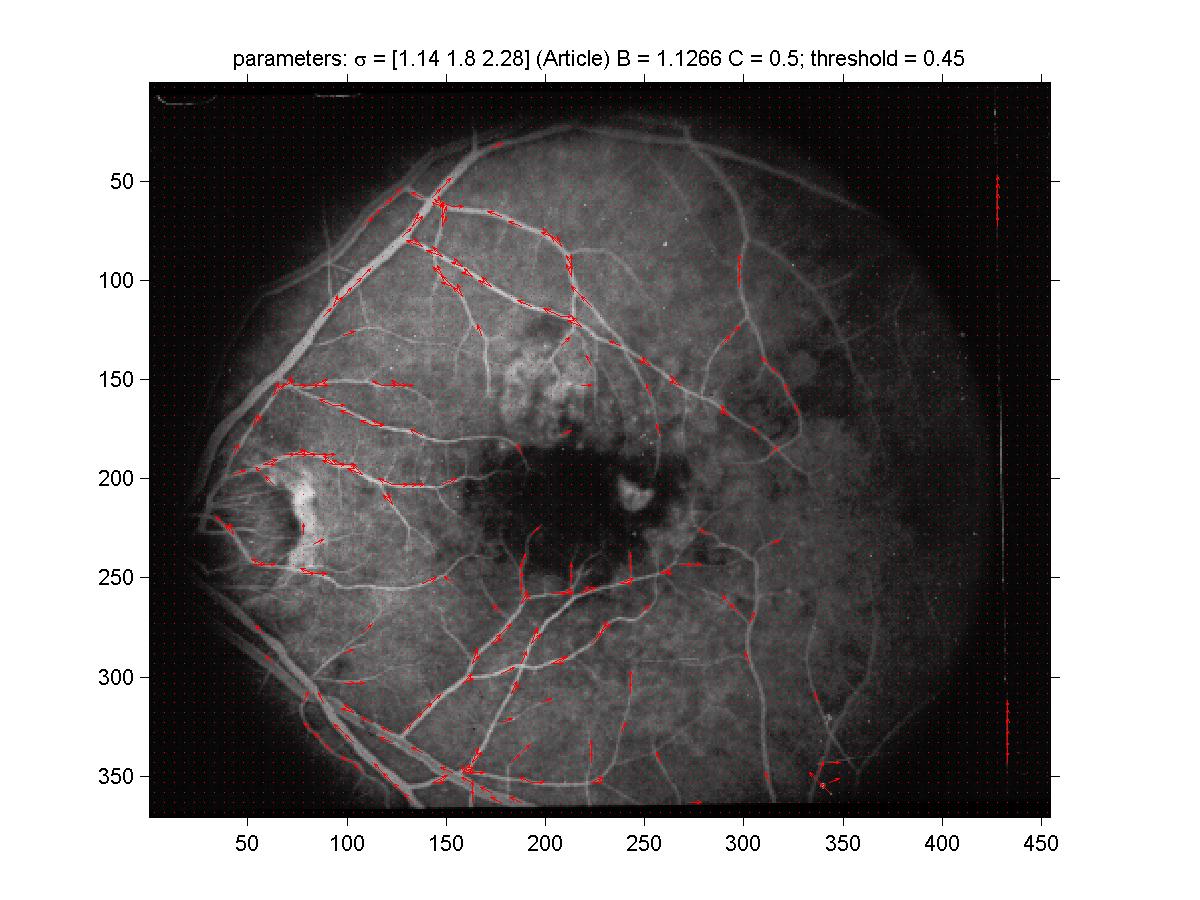 Figure 7: Velocity field arising from kernel of the article. Same
normalization as in figure 6.
Figure 7: Velocity field arising from kernel of the article. Same
normalization as in figure 6.
2.4 Refinements
2.4.1 Thresholding
The first refinement done was about the thresholding. In order to compare the
velocity fields obtained by different methods, we needed a more systematic way
of deciding the threshold. This appeared to be particularly essential in part 3
where the velocity graph was very sensitive to the threshold value (more
about this in part 3). Also, instead of using the same threshold for all orientation,
specific thresholds would be used for each orientation. This can be justified by a
certain independence between the line detectors at each orientation, so that each
orientation can be treated independently in some sense (as we do partially in part 3
with the relaxation labelling method on a network of graphs (one graph per orientation)).
In any case, the different thresholds will be essential in part 2 and 3.
The systematic way of finding a threshold was the following: for each orientation, a loop
is started which counts the number of pixels with a tangent confidence greater than a certain
value (initialized to the mean of the image). The loop iteratively increases the threshold
until the number of surviving pixels drop below a certain number (which determines the density
of surviving vectors that you want; I found that 5000 gave nice results in this experiment).
The threshold precision was 0.001 for my first experiments, and 0.0001 for part 3 when
it appeared that the results were very sensitive on the threshold. The velocity
field obtained by this method is shown in figure 8. Note that the individual
tangent thresholds varied between 0.50 and 0.56, so were similar than the one used in
figure 6. Also, the surviving tangents were a superset of the ones
of figure 6. Finer velocity fields are drawn in figure 9
and figure 10 for two different close-up regions. In this case,
a vector was drawn at each pixel. From those, we see that the tangent estimates
are already quite good, with few noise.
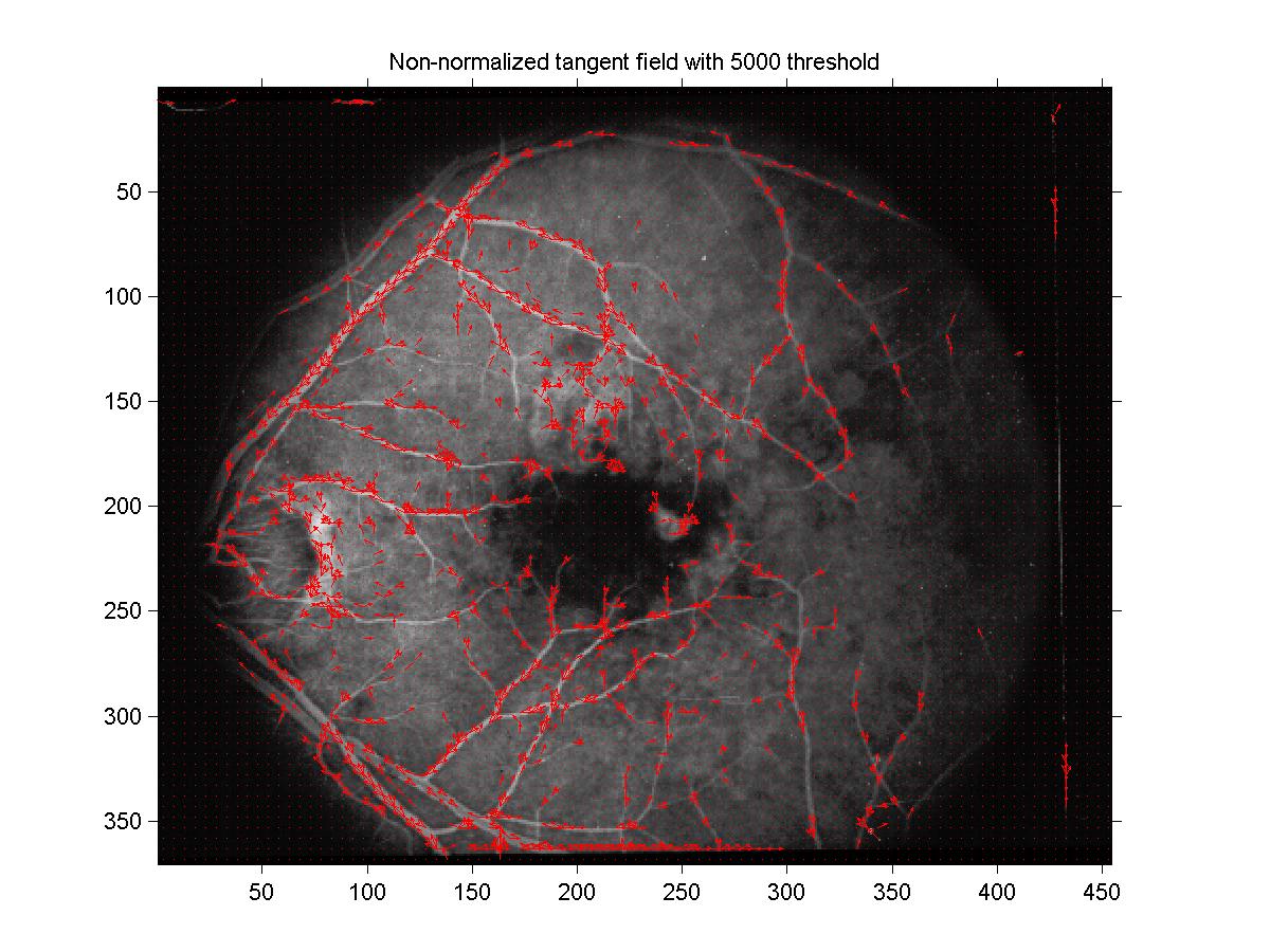 Figure 8: Velocity field with systematic tangent value threshold finding.
The threshold (number of surviving tangents for an orientation) was 5000.
Figure 8: Velocity field with systematic tangent value threshold finding.
The threshold (number of surviving tangents for an orientation) was 5000.
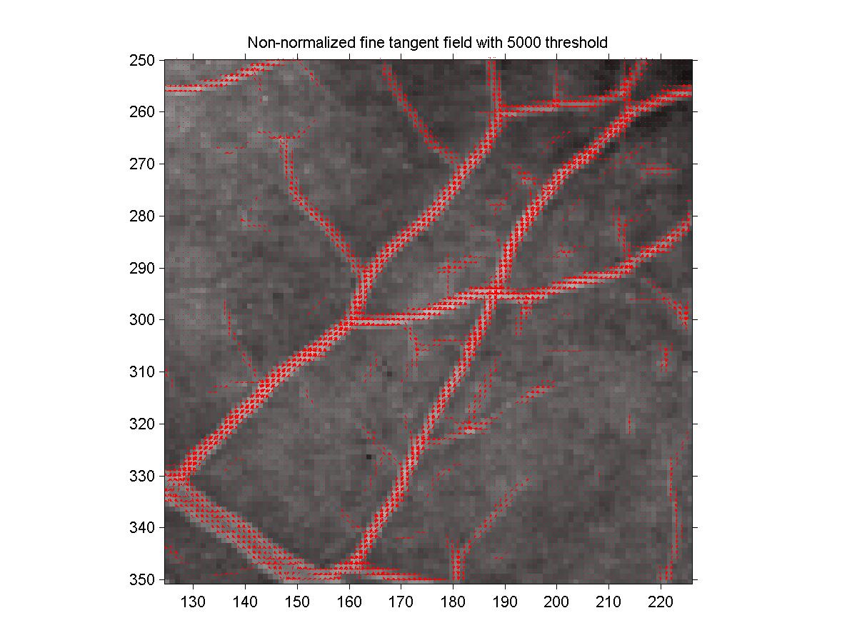 Figure 9: Fine velocity field with threshold = 5000.
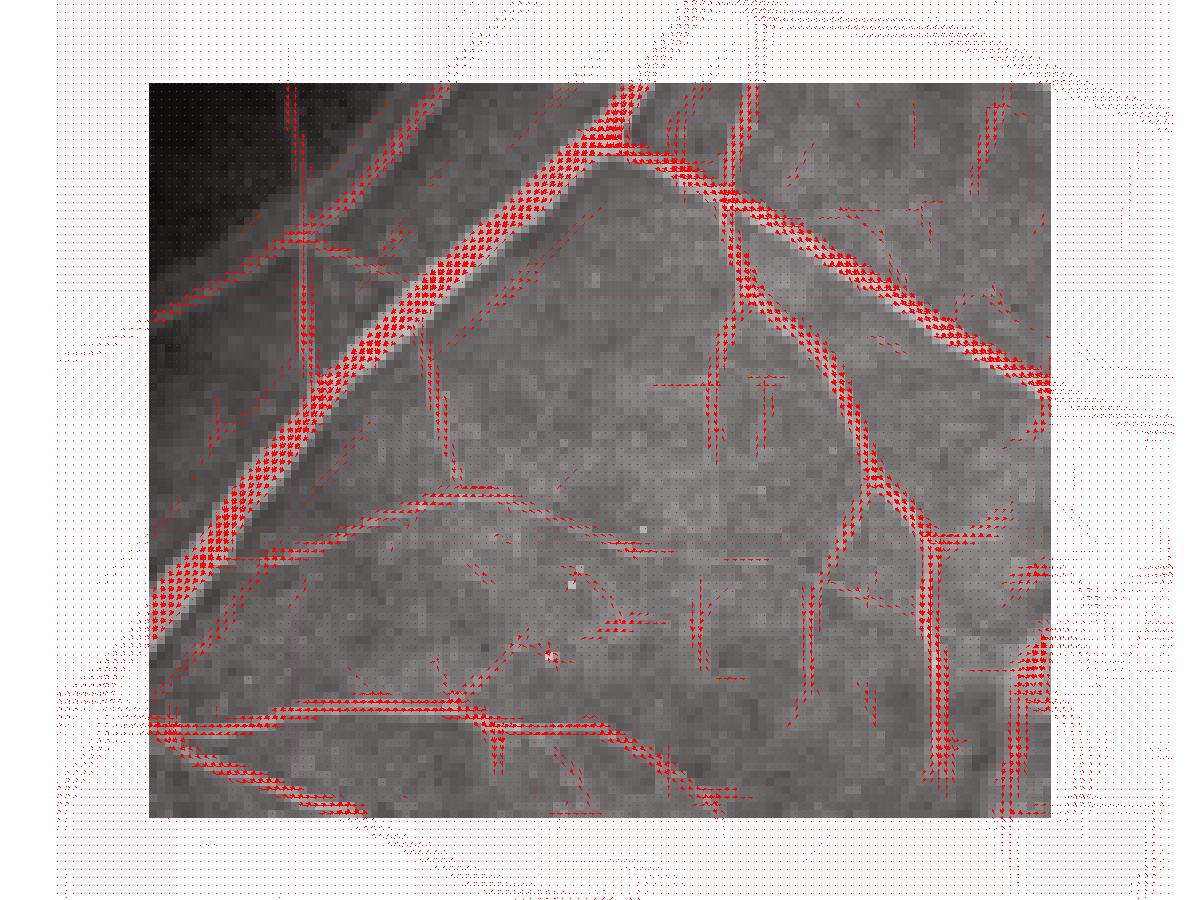 Figure 10: Fine velocity field with threshold = 5000. The zoomed region
was [60, 200]×[60, 180].
Figure 10: Fine velocity field with threshold = 5000. The zoomed region
was [60, 200]×[60, 180].
2.4.2 Normalization
The relaxation labelling method of part 3 uses the assumption that
�l pi(l) = 1. We thus need to renormalize each vector assignment
so that its components sum up to 1. This can be done simply by dividing
each vector by the sum of its components. But it is not necessarily obvious
that what we will obtain as result will be easily interpretable, since the comparison
between each pixel is dimmed by the different normalization of each. That's why
the first experiments I have made simply used a global renormalization, rather
than an individual one. Also, the range of values of most of the assignment vectors
were changed from [0.3 1] to something like [0.125 0.15], so that the difference
between noise and real lines was a lot decreased. Without my systematic assignment
explained in the previous section, the thresholding was really hard, because of the
sensitivity of the number of surviving vectors. Figure 11 and
figure 12 show the new results with this normalization, using
again a threshold of 5000 for an objective comparison with the non-normalized
field. By comparing with figure 8 and figure 9
respectively, we see that the results are similar to the non-normalized version.
The main difference is that the normalized velocity field contain in addition
a lot of perpendicular components close to the vessels, presumably due to
a second effect of the line detector, and the enlarging of the noise because
of the renormalization (before, this signal was just too dim to be perceived).
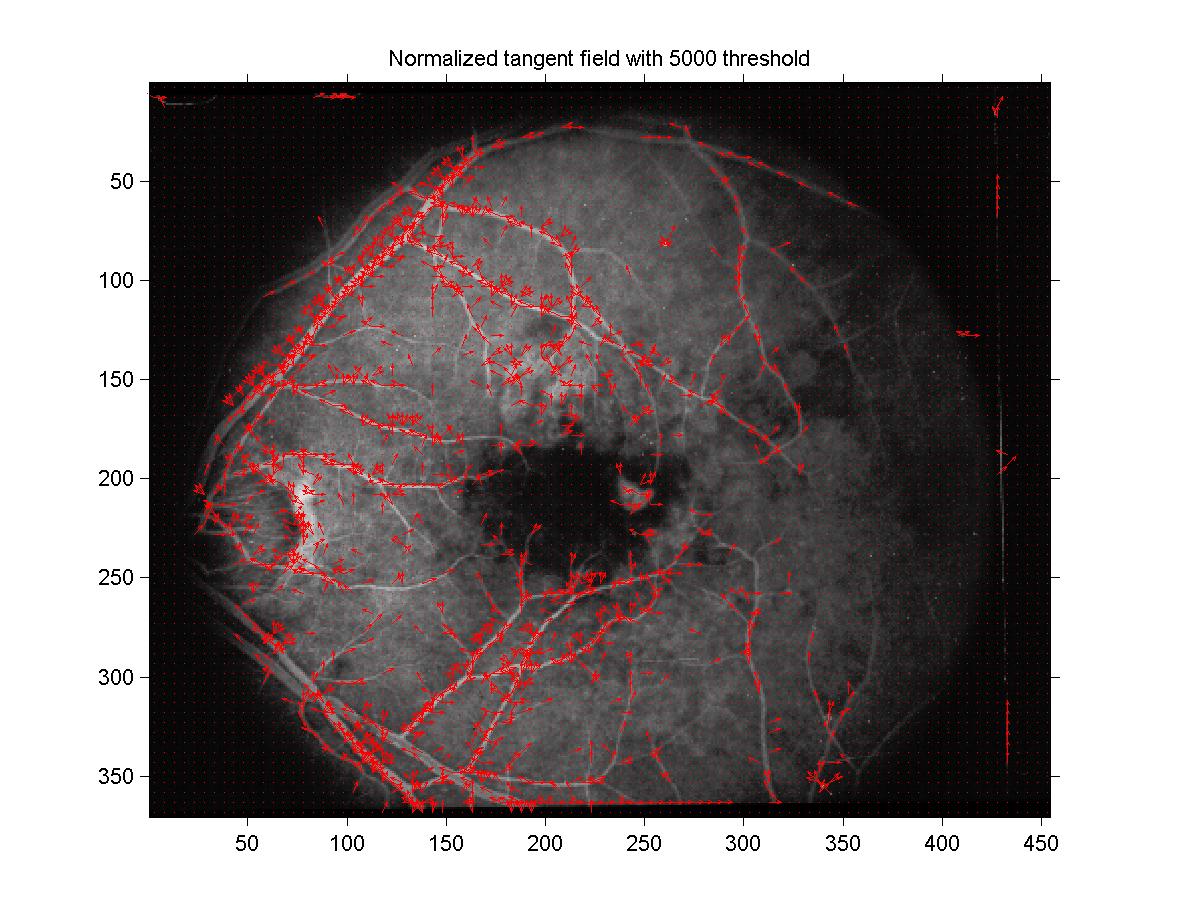 Figure 11: Normalized velocity field with 5000 threshold. 5000 threshold
yielded an individual threshold of roughly 0.14.
Figure 11: Normalized velocity field with 5000 threshold. 5000 threshold
yielded an individual threshold of roughly 0.14.
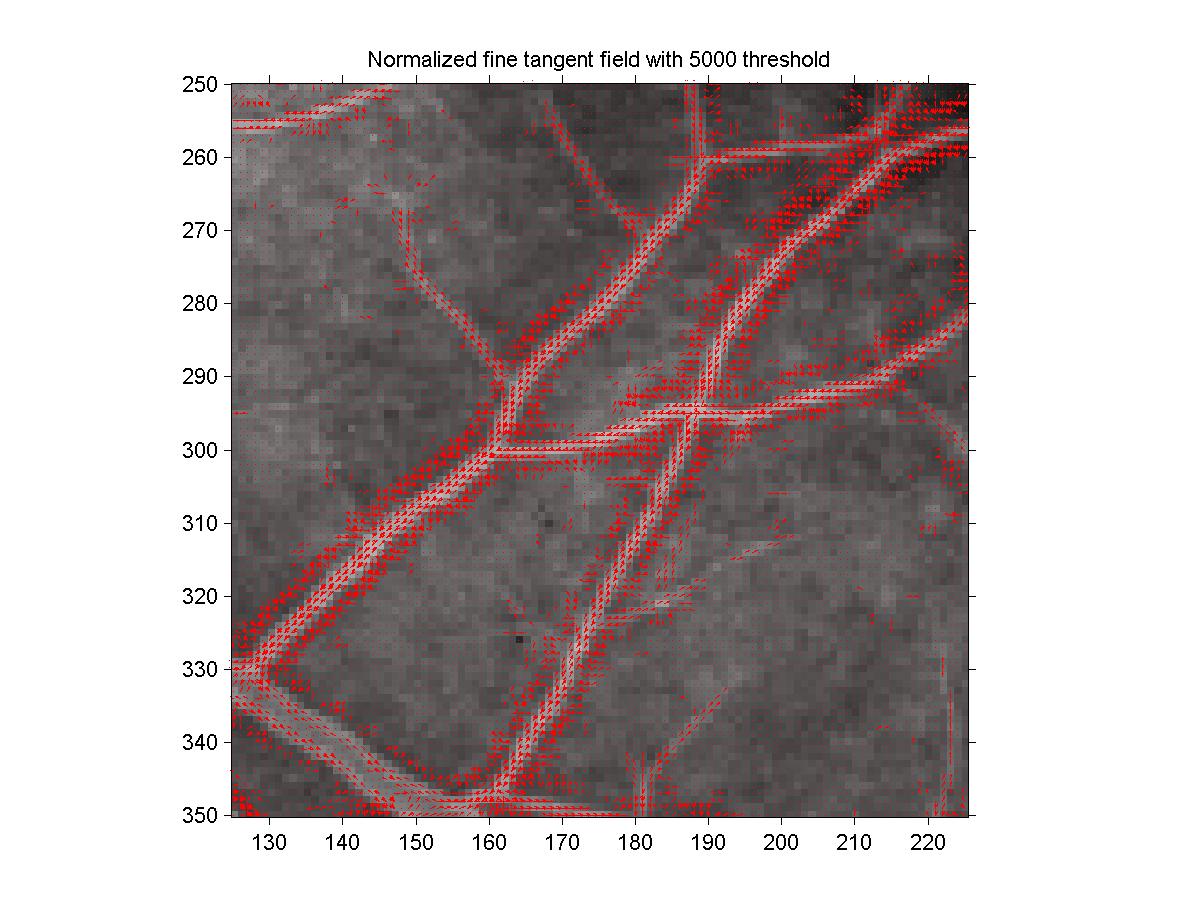 Figure 12: Normalized fine velocity field with 5000 threshold.
3 Part II: Co-Circularity Support
3.1 No curvature class
My first implementation of compatibility didn't include the curvature
classes part. The support function was thus the following:
|
si(l) = |
m
�
l� = 1
|
|
neighbors
�
j=1
|
cij(l, l�) pj(l�) |
| (3) |
as given at the beginning of page 831 in the paper, where cij are the
cocircularity coefficients. It turns out that the cocircularity coefficents cij only depend
on the separation between j and i and not their absolute value. Equation 6
is thus just like a sum of convolutions between the kernel cij and the function pj
(one convolution per l�). This allows us to compute the support very efficiently.
I used again a 15×15 neighborhood to define the kernel cij, assuming that this would
be enough for a first approximation of the support. In my definition of the cocircularity
coefficient, I have not used any linear interpolation (like they did in equation (5.6) of
the article): the value of cij(l, l�)
was simply 1 if l at i was cocircular with l� at j (i.e. if
|
| G(ql, qij) - G(qij, ql�) | < e+ 2a |
| (4) |
as given in equation (5.5) in the article), 0 otherwise. In our case,
e = p/8 and a = sin-1(1/dij),
again using the notation of the article. Finally, qij = tan-1(Dy / Dx)
and G is given in equation (5.3) of the article.
So, taking i to be fixed at the center of a 15×15 neighborhood, I could compute the value
of cij for each l and l� in terms of its position (x,y) in the neighborhood.
An example of such a matrix (for l = l� = 5) is shown in figure 13.
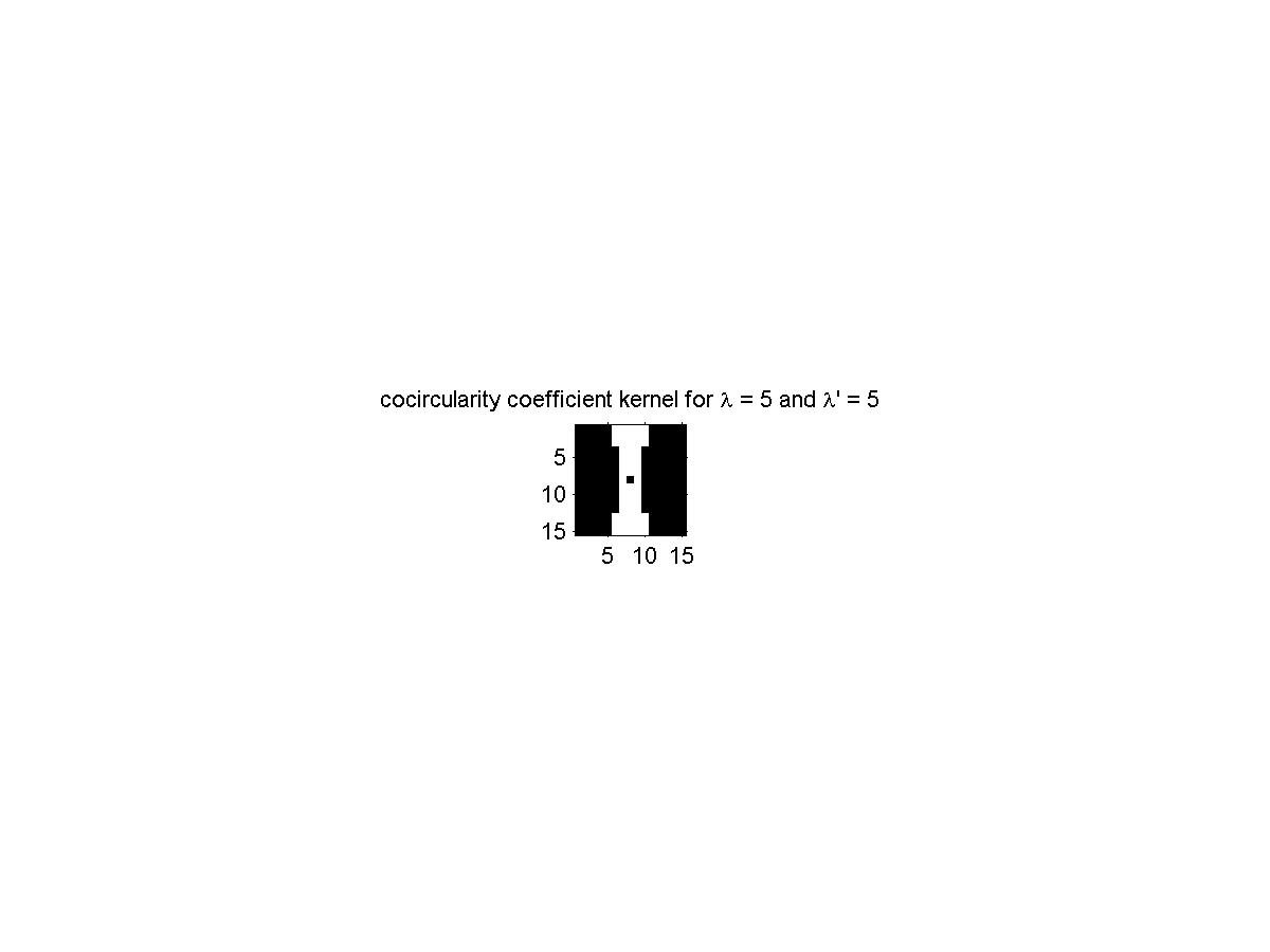 Figure 13: Cocircularity kernel matrix for l = l� = 5 (this is 90o).
White corresponds to 1, black to 0. Note that the center is always 0, since
we don't consider self-interaction in the support.
Figure 13: Cocircularity kernel matrix for l = l� = 5 (this is 90o).
White corresponds to 1, black to 0. Note that the center is always 0, since
we don't consider self-interaction in the support.
Thus, using again filter2 in Matlab, I have convolved cij(l, l�)
with pi(l) (using the normalized ones obtained in part I)
for each l�, and then summed them up to obtain si(l).
This could be done in roughly 15 seconds on my Windows XP Athlon 1.5 GHz 512 MB RAM workstation
at home.
Using the same technique as in part I, I have plotted a velocity field using the assignments
si(l), using the systematic threshold finding, but with a different
normalization: I simply divided si(l) by maxi si(l), for each l.
This yielded values smaller than 1 (and still positive since the kernel was positive).
The normalization depending on l was needed because of the lost of the angular
symmetry which arose from the choice of a rectangular neighborhood. Indeed, the diagonal
of the square is bigger than its side, so diagonal angles are favored with respect to
square angles. Thus, si(l) was systematically bigger for diagonal angles than
for square angles. In any case, the results are shown in figure 14
and figure 15. If we compare them with figure 8
and figure 9, we find that they are not quite different, apart
that the support fields contain a little more junk close to the vessels, but less
noise far from the vessel (the junk appearing at the boundary of the image
could be due to an artifact of the convolution at a boundary).
 Figure 14: Support field with no curvature classes.
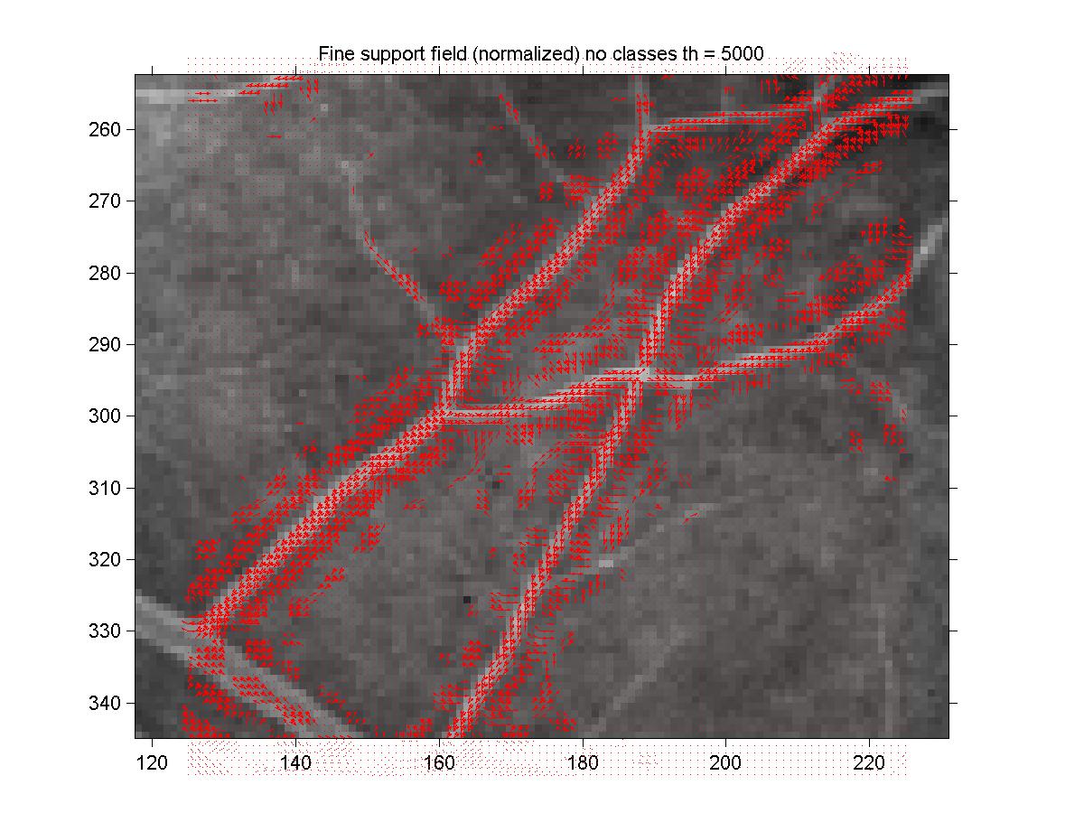 Figure 15: Fine support field with no curvature classes.
3.2 With Curvature Classes
Here, I have added the curvature classes support, but not with
the curvature consistency, due to time constraints. From equation
(5.7) in the article, we can compute the curvature estimate of
each point in the neighborhood in function of l:
|
kij(l) = |
2 sin | G(ql, qij) |
dij
|
|
| (5) |
To find the sign of the curvature, I have used the convention that if you draw a line
in the direction of the tangent (l) at the center of the neighborhood, then
everything which is to the right of it is positive, and negative to the left.
Geometrically, in the upper part of the neighborhood, this amounts to set the
curvature positive when ql � qij.
Figure 16 shows an example of the sign assignment when we consider
the tangent at 167.5o.
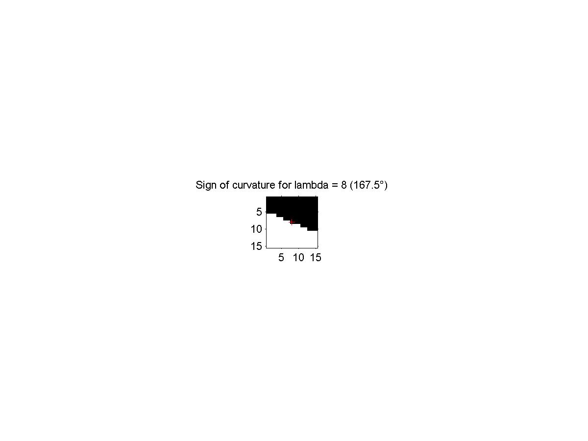 Figure 16: Sign of the curvature region for l = 8. Black is positive,
white is negative.
Figure 16: Sign of the curvature region for l = 8. Black is positive,
white is negative.
With the observation that the vessels don't bend too much, I have decided to use only 3
curvature classes as a first approximation. The limits of the curvature classes were
chosen so that they are not too wide, neither too narrow... Figure 17
shows them.
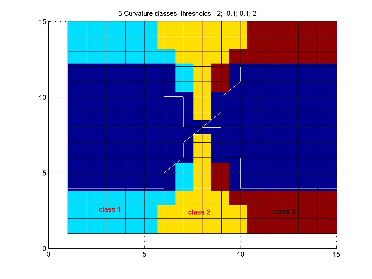 Figure 17: Choice of curvature classes. The 3 classes are: ]-2,0.1],
]-0.1,0.1[, [0.1,2.0[.
Figure 17: Choice of curvature classes. The 3 classes are: ]-2,0.1],
]-0.1,0.1[, [0.1,2.0[.
With the curvature classes, but without the curvature consistency, the support function
becomes:
|
si(l) = |
max
k=1...3
|
|
m
�
l� = 1
|
|
neighbors
�
j=1
|
Kkij(l) cij(l, l�) pj(l�) |
| (6) |
where Kkij(l) is the curvature class coefficient. The resulting support fields are shown
in figure 18 and figure 19. By comparing with the fields without
curvature classes, we see that some tangents have disappeared. Also, we can also see the effect
of the angular asymmetry of the neighborhood by the domination of the diagonal angles in the
resulting support field. One partial solution to this problem is to use a circular neighborhood
(i.e. put 0's outside of a circle to fill a rectangle). I haven't had the time to really experiment
it, though. Other refinements for the angular symmetry are also given in section VI D of the article.
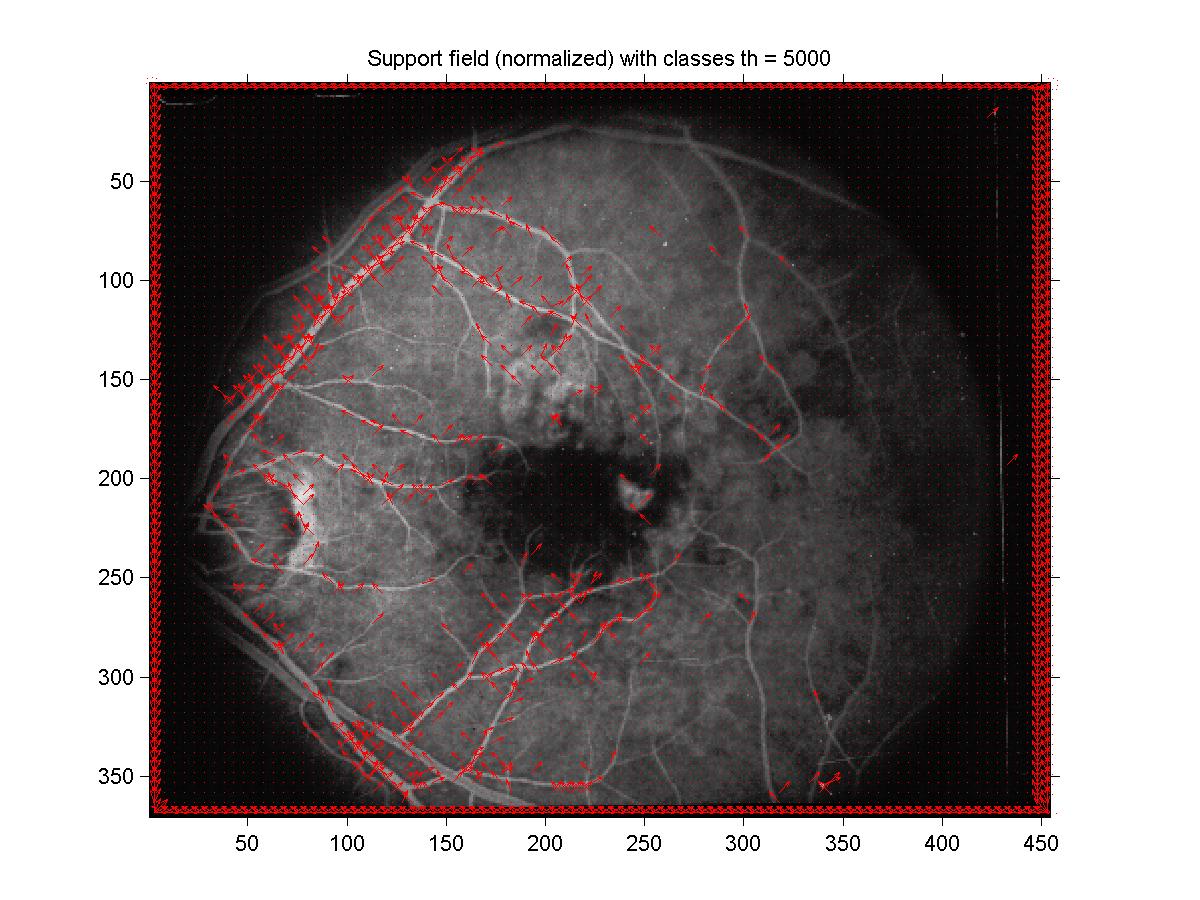 Figure 18: Support field with curvature classes.
Figure 19: Fine support field with curvature classes.
4 Part III: Relaxation Labelling
Using the relaxation labelling method, we can obtain a consistent labelling
(which is defined in equation (A.1) in the article). Equation (A.2.d) relates
the assignment vector at the step k+1 in terms of the
assignment vectors and support vectors at step k1
which is called the radial projection and which is a modified version of
gradient descent for the average local support function. Using the normalized
tangent assignments of part I and the support of part II (but without the curvature
classes, since I found that the classes were not really a success because
of their lack of angular symmetry), I have implemented relaxation labelling.
If I define the error
on the consistency by using the max norm of the difference between the LHS and
RHS of equation (A.1), then it happened that the error would decrease roughly
by a factor of 10 by each step (for example, it passed from 10-1 to
10-6 in 5 steps in my implementation). I will show the results for the
the two first steps. Because of the borderline effect of the convolution
(which I could have solved by shrinking the region of convolution at each
iteration), strong tangent assignments have appeared at the boundary of
the image and so instead of using a threshold of 5000, I have used
a threshold of 15000 in order to see something interesting inside
the image (since most of the count came from the border). The tangent
estimates are plotted in the following figures for the two first steps
(with also the original configuration shown). What we can observe is
that the tangent estimates seem to get more localized after the iterations,
but this could be due to the fact that most of the tangents (to get a
count of 15000) are getting on the border. Also, by looking at the fine
version, we see that layers of tangents appear close to the vessel. I think
that those appear because of the normalization which enhances some noisy
artifacts. Something which is important to mention at this point is that
the sensitivity on the threshold increases significantly as we iterate.
It seems like if each iteration would bring most of the tangent estimates
closer to each other so that we would need a very fine threshold resolution
in order to differentiate the background noise to the real line signal.
That's why I have needed 0.0001 resolution for the thresholding here (a 0.001 was
big enough to switch from 100000 tangents to few hundreds tangents!).
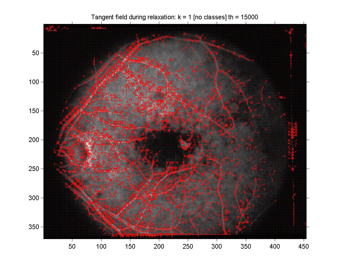 Figure 20: Tangent field at beginning of relaxation.
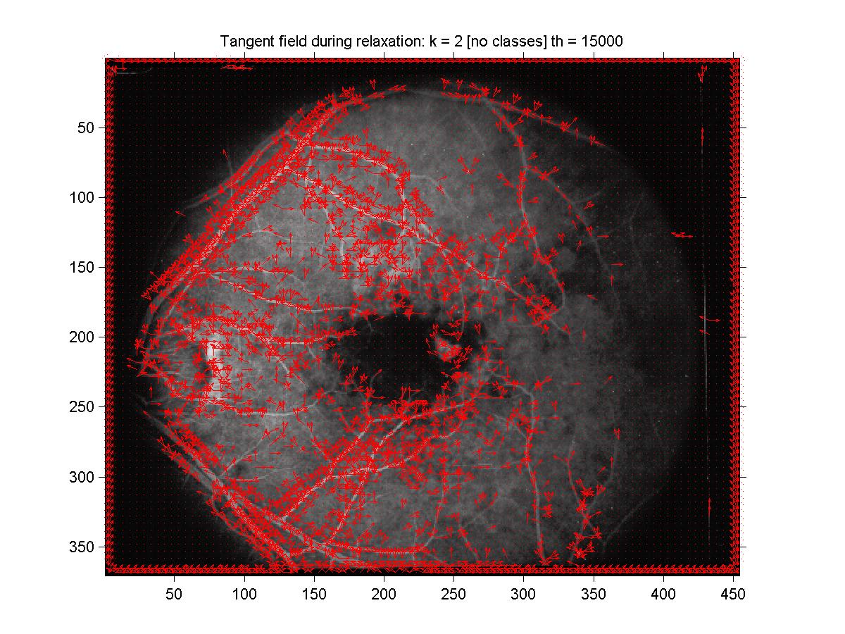 Figure 21: Tangent field after one step of relaxation.
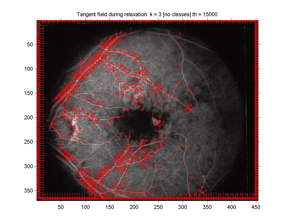 Figure 22: Tangent field after two steps of relaxation.
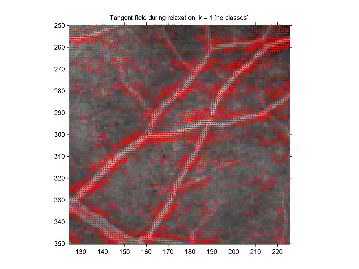 Figure 23: Fine tangent field at beginning of relaxation.
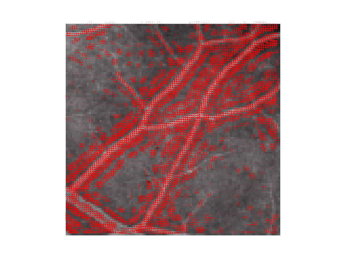 Figure 24: Fine tangent field after one step of relaxation.
Figure 25: Fine tangent field after two steps of relaxation.
5 Conclusion
My implementation of relaxation labelling didn't seem to succeed very
well to get a better set of tangent estimates for the vessels.
The original set of tangent estimates arising from line detection
seemed to be already nice, and wasn't really improved by the local support
information. My hypotheses are that this is due because of the lack of
symmetry of the neighborhood used to compute the local support, and also
because of the normalization of the tangents which seem to increase
the noise instead of clearing it. Indeed, this normalization issue enlarges
a lot the effect of the asymmetry the setting. It is probable that we would
obtain better results by using the relaxation labelling method with
a bigger neighborhood (for the local support calculation) which would also
be spherically symmetric. I have to say that it was very hard to implement
the method of the article. First of all because of many technical details
which needed to be considered. And also because the article didn't explain
well how the normalization should be carried on, even if this has a significant
impact on what you can display.
Footnotes:
1There is no need
in this case to define [s\vec]i*(k) since the support function
is always positive.
File translated from
TEX
by
TTH,
version 3.11.