Final Project Report: Geometrical Analysis of an Area Minimization
Flow and Formalization of its Gradient Descent
April 28, 2003
Simon Lacoste-Julienf
fSchool of Computer Science
McGill University
ID no: 9921489
email: simonlacoste@videotron.ca
Abstract
We present a review of the literature about active contours and gradient flows.
Several mathematical claims have been made about those, and one of the main
subject of this project has been to formalize and justify those claims.
The two main contributions of this project were to clarify and modify
the treatment made by Siddiqi et al. in [15]
about a gradient flow which minimized a weighted area functional
but appeared to be not geometrical;
and to formally justify the notion of gradient descent to derive
gradient flows using the variational derivative and a suitable
inner product defined on the metric space of functions.
Contents
1 Introduction
2 Context of the weighted area minimization flow
2.1 Active contours
2.2 Geometric flows and level sets approach
2.3 Gradient flows
2.4 f-area minimization flow
3 Analysis of the f-area minimization flow
3.1 Geometrical discrepancy
3.2 Corrected flow
3.3 General f-area gradient flow
3.4 Analysis of the doublet
3.5 Impossibility of a general doublet
4 Formalization of gradient descent
4.1 Not all norms are equal
4.2 Justification of gradient with a natural norm
5 Conclusion
1 Introduction
The motivation for this paper has been to try to formalize and justify
some claims which were made in the field of computer vision and which
had puzzled the author for some time. The starting point has been
the article by Siddiqi et al. [15], in which
a new gradient flow for shape segmentation was derived by minimizing
a weighted area functional, with image dependant weighting factor,
in a similar way with what has been done in [9]
by Kichenassamy et al. with a weighted length functional.
The argument in [15] seemed totally geometrical, and yet,
they obtained a curve evolution flow which depended on the origin
of their coordinate system. In this project, we have investigated
the origin of this discrepancy and have tried to obtain a similar
flow which would be truly geometrical. This has lead us to
bring several corrections to the claims made in [15],
and conclude that no simple weighted area functional could
have the behaviour that they had been looking for with their
(wrong if applied without care) gradient flow. We have
conjectured that the geometrical version of the flow could be
still successful in segmenting images under certain conditions.
We have finally investigated a formalization of the meaning
of the 'steepest descent' method which is often briefly stated
in papers in gradient flows, but to which we never found any
formal justification of the terminology. We found that the choice
of the metric in the abstract space of curves is crucial to give
a proper meaning to the method, and that a very natural
inner product gave a solid justification to the terminology,
(``direction of greatest descent'') even in a global sense.
The paper is organized as follows. In section 2,
we give an overview of a selection of the literature related to the area
minimization flow, starting from the active contours article
by Kass et al. [8].
In section 3, we give an analysis and correction of the claims
made by Siddiqi et al. in [15]. We give a corrected
geometrical flow in section 3.1, a general formula
for the weighted area minimization flows in section 3.3
and an analysis of the doublet term in sections 3.4 and later.
Finally, we formalize the notion of gradient for the functionals
appearing in gradient flows in section 4.
2 Context of the weighted area minimization flow
2.1 Active contours
The original (classical) framework for curve evolution
in shape segmentation came from the article by Kass et al. [8]
where they have defined the notion of snakes or active contours.
Their motivation was to provide a unified framework for different visual problems,
including shape segmentation, motion tracking and stereo matching, using
an energy-minimization formulation. The setting was to let evolve
energy-minimizing splines on the image, guided by external constraint forces
and where the energy functional was defined in such a way that the curve
had certain geometrical properties (such as smoothness) and would be attracted
towards features of interest (such as the boundary of an object). A typical
example of energy functional for shape segmentation was
|
E( |
�
C
|
) = a |
�
�
|
1
0
|
| |
�
C
|
p
|
(p)|2dp + b |
�
�
|
1
0
|
| |
�
C
|
pp
|
(p)|2dp - l |
�
�
|
1
0
|
|�I[ |
�
C
|
(p)]|dp |
| (1) |
where [C\vec](p):[0,1]� \mathbbR2 is the parameterized planar
snake, I:[0,a]×[0,b] � \mathbbR+ is the image in
which we want to detect the object boundaries and a, b and a
are real positive constant parameters. The two first terms of equation
control the smoothness of the contours to be detected (and is considered to be
internal energy), while the third term is a potential well which will have
minimal value when the snake is on a high-gradient locus in the image, normally
indicative of an edge (and which is called external energy since it depends
on the image and not the curve).
This provided a more flexible and more global (higher level) approach
to the shape segmentation problem than the previous approach of
detecting edges (using gradient threshold, for example) and then
linking them. The formulation of the problem made it easier to develop
semi-automatic methods for shape segmentation, by having a user doing
minimal interactions with the tool which evolved the contour to capture
the shape of an object. Also, some numerical methods were available
to perform a minimization heuristic of the functional (using gradient
descent). Finally, the energy-minimization concept is a ubiquitous
concept which was used in physics first and then in all branches
of science to model the world around us in a simple way.
2.2 Geometric flows and level sets approach
On the other hand, the original snake formulation had several problems.
First of all, its Lagrangian formulation (evolving the curve directly)
made it hard to handle topological changes in the curve (curve splitting
or merging to handle multiple objects). Also, the energy functional
depends on the parameterization of the curve, and thus is not geometrical.
One would expect the shape segmentation problem to be totally geometrical
(unless that different parameterizations could be thought to represent
different interpretations, or different point of views; but that is another
story), in the sense that it shouldn't depend
on the way we choose our coordinate system (this crucial point will be
stressed again in section 3.1). Equation
failed for this aspect.
Caselles et al. presented in [1] a different model
for shape segmentation based on the geometrical PDE:
|
|
�u
�t
|
= |�u| div |
�
�
|
�u
|�u|
|
�
�
|
|
| (2) |
which describes the motion of the levels set of the function u(x,t),
{x � \mathbbR2: u(x,t)=0}. In fact, if we define a family of
curves [C(p,t)\vec]:[0,1]×[0,T[ � \mathbbR2
which match the levels sets of u(x,t) = 0,
the above PDE can be shown to be equivalent to the curve evolution
equation
where k is the curvature of the curve and [N\vec] is its unit inward normal.
This is the Euclidean curve shortening flow1,
which has been studied in more details in [4] and in [5] by Gage,
amongst others, where its nice geometrical properties (smoothness, inclusion invariance
and shrink to round points) have been exposed.
The level set formulation for the curve evolution permits to switch to a Eulerian perspective
which permits the handling of topological changes quite naturally. The book by
Sethian [14] gives a complete coverage of the level set approach and its
numerical implementation.
In order to do shape segmentation, they modified with
an image dependent term f([x\vec]) and constant positive speed v:
|
|
�u
�t
|
= f( |
�
x
|
) |�u| |
�
�
|
div |
�
�
|
�u
|�u|
|
�
�
|
+ v |
�
�
|
|
| (4) |
where f([x\vec]) is such that it goes to 0 near an edge so that the
level set curve will stay stationary near edges. The one they used was:
|
f( |
�
x
|
) = |
1
1+ (�Gs *I)2
|
|
| (5) |
where Gs *I is the convolution of the image with a Gaussian
kernel of standard deviation s. More recent work used
anisotropic smoothing instead (see [15]) for example, in order
to preserve edges. As edges are normally assumed to be found where the
intensity gradient is high, such a f goes to 0 (or to its minimal value)
near an edge. The constant v term in equation
was added in order to permit the segmentation of non-convex shapes.
Apart solving the topological handling problem using the Eulerian perspective,
their flow was intrinsic or geometric in the sense that it didn't
depend on a specific parameterization, but rather on the geometry of the
image, and thus solved the weaknesses of the snake approach.
Also, the PDE formulation has the theoretical advantage of coming
with a huge literature about existence and uniqueness of solution
theorems, as well as powerful numerical solution techniques.
The article by Malladi et al. [12] gave
the numerical implementation details of the solution to .
We note that because of the discontinuity of when
�u = 0, the existence and uniqueness analysis of the solutions are
made using viscosity analysis, which starts with weaker solutions
and match them with other possible solutions under specific conditions
(see [10] for example). There is now a rather exhaustive
modern treatment of geometrical PDE for image analysis which can be
found in a book by Sapiro [13], and which contains
much of the review made in this paper.
2.3 Gradient flows
Caselles et al. in [2][3]
and, independently, Kichesanassamy et al.
in [10][9] proposed a new active contour
model which unified the geometric flow approach described in
section 2.2 with the classical energy minimization
approach with the snakes. Their approach was motivated by
the derivation of the Euclidean curve shortening flow which arises when
doing gradient descent on the length functional of the curve
(again, this terminology will be made clearer in section 4).
Namely, by defining the f-length functional (with a different notation):
|
Lf(t) = |
�
�
|
L
0
|
f( |
�
C
|
(s,t) ) ds |
| (6) |
where f was the same function as usual defined on the image,
and differentiating with respect to time (assuming a family of curves [C\vec](p,t)
which is C2,1), they obtain (after one integration by parts and lots of manipulation):
|
Lf�(t) = - |
�
�
|
L
0
|
|
�
Ct
|
�[fk- �f� |
�
N
|
] |
�
N
|
ds |
| (7) |
to which someone who is not too rigorous will just say that to maximize the rate of decrease
of Lf, you need:
|
|
�
Ct
|
= [fk- �f� |
�
N
|
] |
�
N
|
|
| (8) |
and you will call this process `to move [C\vec] in the direction of gradient', like
in the steepest descent technique (that's why you will call this flow a gradient flow).
The first term of equation
is the same as the first term which was found in
(but the latter was in level set notation), thus deriving a part of the
geometrical flow as a gradient flow. The second term (which arises naturally in their formulation)
is what they call a doublet term because it makes the curve oscillate around an edge.
Indeed, since edges are located at the minima of f, �f points away of edges
so that -�f�[N\vec] will be positive when [N\vec] points towards
an edge, and thus the curve evolves always towards an edge if fk is
small enough near an edge.
The derivation we just gave was the one from Kichesanassamy et al. [10][9].
The approach by Caselles et al. [2][3] was different
in formulation (and more complete), but yielded the same result
(same flow). Caselles et al. started directly from the snake energy of
equation with b = 0
and with |�I[[C\vec]]| replaced by the more general
-f( |�I[[C\vec]]| ), and reduced the problem of its minimization
to the one of minimizing . The relation was made by
transforming the integrand of to a Lagrangian (we now use the Lagrangian
mechanics terminology). The energy integral then represents the action,
and thus minimizing the energy amounts to minimizing the action.
They then use the Maupertuis' Principle (see [7]), to relate the curves with
least action to the geodesics with a new Riemannian metric. The metric they need
is precisely f, and thus the geodesics (which minimize length) in this Riemannian
space minimize the f-length functional given by , and thus
yield the same gradient flow equation .
This beautiful relationship can be even extended in a comparison with
the theory of General Relativity: in this case, a metric is defined in
function of the distribution of mass, and the trajectory of particles
is found by the minimization of the action, which depends on the metric.
In our case, the metric is defined as a function of the gradient of intensity
in the image, and the trajectory of the contour is found by minimizing
the weighted length functional.
2.4 f-area minimization flow
Even if the doublet term in equation gives some additional
strength to the flow (which can thus becomes non-convex), when the curve is far
from the edges (so that �f is small) and the enclosed region is big (like at
the beginning), so that k is small, then the flow evolves very slowly.
This is why a constant term fv
(constant in the sense that it doesn't depend on the curve) is still added
in the flow of equation
in practice. Caselles et al. formalized this part of their flow as a
Lagrange multiplier which would arise in a geodesic problem with constraint (they
haven't been explicit about which constraint, though).
The main contribution of Siddiqi et al. in [15] was to try
to derive the constant term (with f) with a similar functional minimization
argument than what Kichesanassamy et al. used. Starting from the
observation that doing gradient descent on the area functional of a curve
(area enclosed by the curve) yielded a constant flow [C\vec]t = [N\vec]
as the gradient flow, they decided to parallel the argument of
Kichesanassamy et al. with an area functional. The area enclosed by a curve
is:
|
A(t) = |
�
�
|
|
�
�
|
R
|
dxdy = - |
1
2
|
|
�
�
|
L
0
|
|
�
C
|
� |
�
N
|
ds |
| (9) |
where Green's theorem (divergence theorem in the plane) was used to transform
the double integral as a path integral, since ��[C\vec] = 2.
They now define the f-area functional:
|
Af(t) = - |
1
2
|
|
�
�
|
L
0
|
f |
�
C
|
� |
�
N
|
ds |
| (10) |
and again differentiating with respect to time and evolving in the direction
of the gradient yields the gradient flow equation
|
|
�
C
|
t
|
= (f+ |
1
2
|
�f� |
�
C
|
) |
�
N
|
|
| (11) |
As a small side comment, we note that in their derivation, they said to have dropped
the tangent terms because they could be killed anyway by a suitable reparameterization.
The justification for this claim can be found in [4] or [13,p.72],
where it is proven that any reparameterization of the curve evolution equation
only changes the coefficients in front of the tangent term, and those can be made zero
by solving an ODE which always has a solution for reasonable coefficient function.
But it is useful to note that the tangent terms cancelled anyway in their case.
They then claimed that the second term, �f�[C\vec], acted also like
a doublet term (though weaker), in analogy with the doublet of .
And to support their claim, they showed an experiment in which they evolved a curve
according to the flow (using a level set implementation)
on a toy image with a hole in the boundary. If the hole wasn't too big, the `doublet'
was strong enough to prevent the curve to leak through the boundary.
But sometimes, the strength of this doublet wasn't strong enough so that they
decided to combine both the f-length flow with the f-area flow
to combine the strength of the doublets:
|
|
�
C
|
t
|
= |
f-length
|
+ |
f-area
|
|
| (12) |
where a is said to be a ``fudge'' factor to make the units compatible (area and length).
But it is in fact more than just a ``fudge'' factor, since the above equation can be seen as the
gradient flow on the functional aLf(t) + Af(t) and thus a can also be
interpreted as the weight (importance) of the length contribution in comparison with the
area contribution in the functional to minimize. The few experiments they
show in the paper then shows that their second doublet helps the curve to stick to the boundary
even when there are holes.
But there was something fishy about their flow. First of all, we didn't find obvious
at all that �f�[C\vec] acted as a doublet. The explanation will
be given in section 3.4. But most importantly, the presence of the term
[C\vec] (which is a vector from the origin to the curve) made the flow to appear
as non-geometrical, since [C\vec] depends on the origin for the coordinate system,
whereas all the other quantities [C\vec]t, [N\vec], k, f and �f
are geometrical quantities which depend only on the structure of the image and the curve, and
not on the coordinate system used. Since the flow was said to be derived from a weighted
area functional minimization, and that area is a geometrical quantity, it would be surprising
to obtain a non-geometrical equation as the way to solve a geometrical problem!
Where is the mistake in the reasoning?
3 Analysis of the f-area minimization flow
3.1 Geometrical discrepancy
The answer lies between equation and equation .
Indeed, already equation doesn't seem geometrical because of the presence
of the term [C\vec] in the curve integral. But unless Green's theorem is wrong,
we should expect this integral to be invariant under translation of origin because
area is invariant under translation of origin. Let's do a change of origin,
so that [C\vec] � [C\vec] - [x\vec]0, where [x\vec]0 is the new origin.
Then the f-area transforms as:
|
|
| | |
- |
1
2
|
|
�
�
|
L
0
|
f( |
�
C
|
- |
�
x0
|
)� |
�
N
|
ds |
|
| | |
Af + |
1
2
|
|
�
x0
|
� |
�
�
|
L
0
|
f |
�
N
|
ds |
|
|
|
|
Now, since [N\vec] = [^k] ×[T\vec], where [^k] is a z-axis unit vector,
we can write the last integral when f = 1 (i.e., the unweighed case):
|
|
�
�
|
L
0
|
|
�
N
|
ds = |
^
k
|
× |
�
�
|
L
0
|
|
�
T
|
ds = |
^
k
|
× | �
(�)
�
| |
�
dr
|
= 0 |
|
since [T\vec] ds = [dr\vec] is the displacement vector, so that the last integral is just
a total displacement around a loop. But if we add the f weight function, the last
integral is not guaranteed to yield zero, and thus the f-area functional that they
had defined was not independent of the origin. The moral of the story is that
we need to be careful with those hidden transformations before making generalizations!
3.2 Corrected flow
In order to correct the flow, all we need to do is to replace the origin dependant
vector [C\vec] by a `true' vector (i.e. independent of the origin). The difference
between two vectors doesn't depend on the origin, and thus we could `fix' some
geometrical origin on the image (like the bottom left corner; or the center of mass
of the image2) and
now measure [C\vec] with respect to this fixed origin. The new f-area functional
would thus be:
|
Af(t) = - |
1
2
|
|
�
�
|
L
0
|
f( |
�
C
|
- |
�
x0
|
) � |
�
N
|
ds |
| (13) |
and we could expect the corresponding gradient flow to be:
|
|
�
C
|
t
|
= (f+ |
1
2
|
�f�( |
�
C
|
- |
�
x0
|
) ) |
�
N
|
|
| (14) |
which is now geometrical. Instead of proving that this is indeed the gradient
flow that we obtain from , we will use a special case of
the general derivation of the gradient flow for f-area functional in the next section.
3.3 General f-area gradient flow
Another critique that we had about their formulation of the f-area is that because
the weighted function f was added in the curve integral rather than the double
integral, it lost its direct metric interpretation which was so nice in the
paper by Caselles et al.. In order to recover it, we will define the
general y-area functional:
where y here has now a true metric interpretation. We now assume that y is
a function of position only in the image (and not of the boundary of the region
of integration). We will compute its first variation by two different means. The first one
is simplest and has a nice geometrical interpretation, but it doesn't link
with . Figure 1 shows the variation of the region after a time
dt when the boundary evolves with speed [C\vec]t(s).
 Figure 1: Variation of area region
The difference between the two
region can be made by adding all the infinitesimal element of area formed by the infinitesimal
vectors [C\vec]tdt and [T\vec]ds (those will be added along the boundary, and thus it
will be a curve integral). The area enclosed by those two vectors is simply
their cross product:
|
dA = | |
�
C
|
t
|
dt × |
�
T
|
ds| = |( |
�
C
|
t
|
� |
�
N
|
) |
�
N
|
dtds| = |( |
�
C
|
t
|
� |
�
N
|
)dtds| |
|
where the second equality was made by expanding [C\vec]t in the orthogonal basis [T\vec],[N\vec]
and the last equality used the fact that [N\vec] was a unit vector. We can assume that y
is roughly constant on the small element of area (for dt small enough), and thus the variation
can be written (keeping the sign right):
|
Ay�(t)dt = Ay(t+dt) - Ay(t) = - |
�
�
|
L
0
|
y |
�
C
|
t
|
� |
�
N
|
dsdt |
|
and from this we conclude that the gradient flow equation is simply
where we recover the usual constant normal flow in the case in which we minimize the Euclidean area.
We now give another derivation for this simple result. Given a reasonable function
y([x\vec]), we define a vector field [F\vec]([x\vec]) such that
This is a simple Poisson equation which can be solved in theory for any reasonable y.
For a specific form for [F\vec], we use Helmoltz theorem (see [6]):
|
|
�
F
|
( |
�
x
|
) = -� |
�
�
�
�
|
1
4p
|
|
�
�
|
|
�
�
|
|
�
�
|
|
|
d3x� |
�
�
�
�
|
|
| (18) |
where the integral is taken on the whole space. The physicist will recognize on the right the gradient of the
electric potential formula. Anyhow, this integral gives us the required vector field. We can now
transform using the divergence theorem in the plane:
|
Ay(t) = |
�
�
|
|
�
�
|
ydA = |
�
�
|
|
�
�
|
�� |
�
F
|
dA = - |
�
�
|
L
0
|
|
�
F
|
( |
�
C
|
) � |
�
N
|
ds |
| (19) |
where the minus sign comes from the fact that we use an inward normal. We could compute the time
derivative of this functional, as usual, and use some integration by parts, lots of calculus and get
incredible cancellations to obtain
|
Ay�(t) = - |
�
�
|
L
0
|
|
�
Ct
|
�[(�� |
�
F
|
) |
�
N
|
] ds |
| (20) |
and since ��[F\vec] = y, we obtain back equation as our
gradient flow. But instead of giving the details, we refer the reader to the
article by Vasilevskiy and Siddiqi
about flux maximizing flows [16]. They have shown there that the flux maximizing
flow was the one evolving with the divergence of the vector field (as we have just seen).
It is now easy to prove the previous claim about the gradient flow for our geometric
f-area functional . In this case, we see that
[F\vec] = -[ 1/2]f([C\vec]-[x\vec]0). Computing its divergence, we can easily get back
equation .
3.4 Analysis of the doublet
We now investigate if
acts like a doublet. Looking at
figure 2, we see that the magnitude of [C\vec] doesn't change much when a point crosses
a boundary (unless the origin was very close to the point we are looking at), whereas �f
changes sign as expected by the way it was defined.
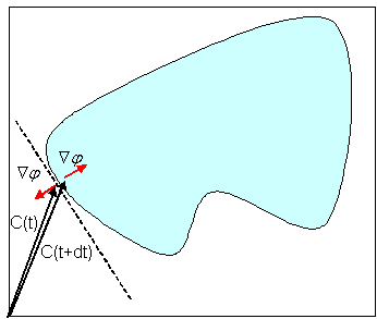 Figure 2: Simili-doublet
This means that �f�[C\vec] will switch sign when crossing the boundary.
We can now see that each edge separates the image in two
(drawn with a dashed line on the figure): when the origin is on the side
of the inward normal of the edge, than the doublet will really acts like a doublet: it will
attract the curve. On the other hand, when the origin is on the other side of the edge
(the outward normal side), the doublet will act like a repulsor. Also, the farther
the origin is from the edge, the stronger is the effect since the norm of [C\vec] enters
in the simili-doublet. This means that for a proper choice of origin, the effect can be quite
strong (and this is what was observed in [15]). It appeared that all the examples
that were used in [15] had the origin on the correct side of the hole in the edge;
and thus they had good results with their simili-doublet. It would have been interesting
to experiment with the flow with different positions of origin.
Unfortunately, we haven't been able to implement this due to time constraint.
In practice, we believe that a good engineering heuristics to make good use of the
simili-doublet is to use a different origin for each curve, and place the origin at the seed
where the curves are started (assuming we use a growing flow instead of a shrinking one).
This way, you maximize your chances that the origin will be on the correct side of the edge
since the curve should surround at first the seed placed. This is something which could be
investigated in the future.
3.5 Impossibility of a general doublet
Finally, we investigate if it is possible to obtain a doublet which would always
work (not depending on the position of the origin),
from a gradient flow of a y-area functional. There are two main components
which a doublet should contain: information about the edge (this is given by �y)
and information about the direction of the curve evolution (this is given by [N\vec]).
This is why the real only general doublet is �y�[N\vec].
Since the speed function of the gradient flow of y-area functional is simply
y, we will need the doublet in the definition of y in order
to obtain it in the gradient flow. The problem is that [N\vec] has meaning
only on the boundary of the region! Since we integrate y over a whole
region, it wouldn't make sense to include a [N\vec] in the integrand
(it isn't defined on the whole region; �f is, though).
This is why we conclude that no simple y could yield
the required doublet as a gradient flow for a y-area functional;
only a f-length functional can yield one.
We could maybe obtain this doublet using a more complex y, though
(defining it as a functional which could depend on the boundary of the region).
This is similar to the problem of speed extension which happens
in the level set approach when the speed has only a meaning on the boundary
but we want to define it on the whole region for the surface evolution
(see [12] or [13,p.83]). An example of such an extension would try to extend
the normal from to the boundary to the region. But in this case, our derivation for
the gradient flow breaks down since we had assumed that y depended
only on position, and not on the boundary. More powerful tools of functional
analysis would be needed to analyze this new gradient flow.
4 Formalization of gradient descent
In this section, we will investigate the formal meaning of the innocently looking
sentence: ``to maximize L�(t), the curve has to evolve in the following
way... which is thus the direction of the gradient''.
We will take as a canonical example the Euclidean curve shortening flow:
which has first variation
|
L�(t) = - |
�
�
|
L
0
|
|
�
Ct
|
�k |
�
N
|
ds |
| (23) |
First of all, the problem of finding [C\vec]t(s) which
will ``maximize'' the integral on the RHS in a global or even local
sense has no meaning by itself, since you can make it as big as you want
by just making |[C\vec]t(s)| as big as you want... But when one wants
to talk about variations and derivatives, one has to use at least the
framework of metric space and thus choose a norm (metric). The functional
L�(t) takes a given function [C\vec]t(s):[0,L]� \mathbbR2
and return a real number. Let's call D[0,L] the set of such functions.
For simplicity, we won't go into the details of how much differentiable
are the functions in our space. But it has to be at least integrable
to make sense.
4.1 Not all norms are equal
What norm should we used in our space? As a starting point (and to
demonstrate the importance of choosing a correct norm), we will
choose the following norm on D:
|
|| |
�
C
|
t
|
|| � |
�
�
|
L
0
|
| |
�
C
|
t
|
(s)| ds |
| (24) |
This norm represents in some sense the total displacement
we would need to move the curve for a unit time dt, and is thus
representative of the work needed. Then in the terminology of
variational calculus, it would make sense to define the gradient
as the `direction' in our space in which the directional derivative
is maximal. And a direction should be unit, otherwise it would contain
more information than just the direction. Thus, to find the gradient
of , we want to find the unit direction [C\vec]t
(i.e. || [C\vec]t|| = 1) which will maximize -L�(t)
(i.e. minimize L�(t)). So WLOG, assume that [C\vec]t = g(s) [N\vec],
for some function g(s) such that || [C\vec]t|| = �0L |g(s)|ds = 1.
then
|
-L�(t) = |
�
�
|
L
0
|
g(s)k(s)ds |
| (25) |
We can now find a bound on -L�(t). Let K = maxs k(s). Then
|
-L�(t) � |
�
�
|
L
0
|
K |g(s)| ds = K |
| (26) |
But unless that k(s) is constant around its maximum value
(for example, in the case of a circle where we have k(s) = K),
then we will never be able to reach this upper bound, but can
get as close as we want by taking g(s) which looks like a dirac-delta
function centered at the position of the maximum of k(s) (see figure 3).
Thus, there is no maximum in this case. Moreover, the usual choice of g(s) = k(s)
that we used in the gradient flows derivation isn't even a local maximum in general
(can move a bit in D[0,L] and still increase its value). Hence we see that with
this norm, the `gradient' doesn't even exist!
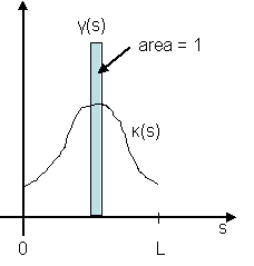 Figure 3: Dirac-delta function to optimize integral.
4.2 Justification of gradient with a natural norm
We now present a natural choice of norm which would justify the method of
gradient descent presented in gradient flows. One key concept is to make
a parallel with the finite dimensional case. For a function f([x\vec]),
we have the differential (variation) for a direction [dx\vec] is:
|
df = �f � |
�
dx
|
= |�f| | |
�
dx
|
|cosq |
| (27) |
where q is the angle between �f and [dx\vec].
And there the maximal value is reached when cosq = 1, i.e. when
[dx\vec] is parallel to �f, and thus, in the direction of the
gradient. To obtain a similar result in a function space, we need to
define an inner product < ·, · > (and from it we can
define the natural norm || v || = �{ < v, v > }).
An obvious inner product to define on D[a,b] is simply:
|
< |
�
A
|
, |
�
B
|
> = |
�
�
|
b
a
|
|
�
A
|
(p) � |
�
B
|
(p) dp |
| (28) |
It is easy to show that this really defines an inner product (with the
equality of functions to be defined as equal essentially
everywhere - i.e. equal everywhere except on a set of measure zero).
From the inner product, we define the norm as usual. With this framework,
let's look at the general problem of extremizing the functional:
|
L[ |
�
u
|
] = |
�
�
|
1
0
|
F( |
�
u
|
(p), |
�
u
|
p
|
(p) ) dp |
| (29) |
where F:\mathbbR2 � \mathbbR and [u(p)\vec] is some function on
[0,1]. The first variation (differential)
of this functional at the point [u\vec] can be written as
|
dL[u\vec]( d |
�
u
|
) = L( |
�
u
|
+ d |
�
u
|
) - L( |
�
u
|
) = |
�
�
|
1
0
|
|
dF
|
�d |
�
u
|
dp = < |
dF
|
, d |
�
u
|
> |
| (30) |
where we have used the notation [( dF)/(d[u\vec])]
to represent the vector [( dF)/(dui)], and where
we have used the variational derivative:
|
|
dF
du
|
� |
�F
�u
|
- |
d
dp
|
|
�
�
|
�F
�up
|
�
�
|
|
| (31) |
which simply represents the Euler-Lagrange equation (see [7]).
The last equality in simply came from our natural definition of
our inner product. But now because of Cauchy-Schwartz inequality, we have
|
< |
dF
|
, d |
�
u
|
> � || |
dF
|
|| ||d |
�
u
|
|| |
| (32) |
with the equality satisfied if and only if [( dF)/(d[u\vec])] is parallel to d[u\vec].
Since the directional derivative of the functional in the direction d[u\vec] is defined as:
|
Dd[u\vec] L � |
1
|
dL[ d |
�
u
|
] |
| (33) |
we have that, using Cauchy-Schwartz:
and thus that ||[( dF)/(d[u\vec])] || is the maximal value of the directional
derivative and the unique directions (up to a global
proportionality constant) in which the maximum is reached is when d[u\vec]
is parallel to [( dF)/(d[u\vec])], and thus
[( dF)/(d[u\vec])] is truly the gradient!
Finally, let's link this variational calculus formalism with the usual curve evolution
framework. We said that was the first variation of .
Indeed, the direction of the variation is simply d[u\vec] = [C\vec]t dt and multiplying
both side of the equation by dt we get:
|
dL = L�(t)dt = - |
�
�
|
L
0
|
d |
�
u
|
�k |
�
N
|
ds |
| (35) |
and thus comparing with equation , we conclude that
(|up| comes from the switch from the parameterization in s to the one on [0,1] on which our
inner product was defined). So we see that we were justified to call -k[N\vec] the
`gradient' of the length functional (using the parameterization in length),
and justify at the same time all the gradient flow terminology.
In summary, we can justify the gradient terminology if we define a proper inner product. In the
first case that we had considered, my norm didn't have a suitable inner product and thus no
gradient could be defined. As a side comment, we note that we recently found a formal treatment
of the gradient descent method on quadratic functionals in [11,p.220].
We haven't had the time to decipher their notation, though, so this would be an investigation
to do in the future...
5 Conclusion
A review of the active contours framework has been presented, starting from the snakes and energy
minimization approach, followed by the geometric flow alternative and their reunification with
geodesic flows or gradient flows. We were then lead naturally to the
article by Siqqiqi et al. [15] about the f-area minimization flow.
Their flow was shown to be not geometrical and an alternative has been suggested, by fixing
the origin in a geometrical way. We have conjectured that a combination of this flow with
the usual f-length gradient flow could be more successful than the f-length
flow alone if the origin was initialized at the same place than the seeds. Some experimentations
are remained to be done to verify that. The simili-doublet term mentioned in [15]
has been analyzed and it was argued that no real doublet term could be derived
in general by minimizing a y-area functional with y not depending on the boundary.
It was suggested, though, that some novel results could be obtained by considering
y as a functional of the boundary rather than a simple function, and the functional
relationship could be similar to the speed extension formulation mentioned in the level set
approach [12]. Finally, we have formalized the meaning of the method of
gradient descent on the simple functionals arising in gradient flows, by defining a natural
inner product which implied that the gradient of a functional is the variational derivative.
It was also shown that other norms defined on the metric space of functions could lead
to very different results (as the non-existence of a gradient).
* Acknowledgements
We would like to thank Kaleem Siddiqi for his supervision, his
patience and also to have endured our critiques... Special thanks to Pavel
Dimitrov and Carlos Phillips for the very helpful discussions we have
had about this project. Many ideas have originated from those
discussions. Another special thanks to Maxime Descoteaux for a workshop
on the numerical implementation of level sets approach which we haven't had
the time, unfortunately, to finish.
References
- [1]
-
V. Caselles, F. Catte, T. Coll, and F. Dibos, ``A geometric model for
active contours'', Numerische Mathematik, vol. 66, pp. 1-31 (1993).
- [2]
-
V. Caselles, R. Kimmel, and G. Sapiro, ``Geodesic active contours,''
ICCV'95, pp. 694-699 (1995).
- [3]
-
V. Caselles, R. Kimmel, and G. Sapiro, ``Geodesic active contours,''
Internation Journal of Computer Vision, vol. 22(1), pp. 61-79 (1997).
- [4]
-
C.L. Epstein and M. Gage, ``The curve shortening flow,''
in Wave Motion: Theory, Modelling, and Computation,
A. Chorin and A. Majda, Editors, Springer-Verlag, New York, 1987.
- [5]
-
M. Gage, ``On an area-preserving evolution equation for plane curves,''
Contemporary Mathematics, vol. 51, pp. 51-62 (1986).
- [6]
-
D.J. Griffiths, Introduction to Electrodynamics, 3rd edition, Prentice Hall,
Upper Saddle River, NJ, 1999.
- [7]
-
L.N. Hand and J.D. Finch, Analytical Mechanics, Cambridge University Press,
Cambridge, U.K., 1998.
- [8]
-
M. Kass, A. Witkin, and D. Terzopoulos, ``Snakes: Active contour models,''
International Journal of Computer Vision, vol. 1, pp. 321-331 (1988).
- [9]
-
S. Kichenassamy, A. Kumar, P. Olver, A. Tannenbaum, and A. Yezzi, ``Gradient flows
and geometric active contour models'', in Proceedings of the International
Conference of Computer Vision '95, IEEE Publications, pp. 810-815, 1995.
- [10]
-
S. Kichenassamy, A. Kumar, P. Olver, A. Tannenbaum, and A. Yezzi, ``Conformal
curvature flows: from phase transitions to active vision'',
Archive for Rational Mechanics and Analysis, vol. 134, pp. 275-301 (1996).
- [11]
-
V.I. Lebedev, An Introduction to Functional Analysis and Computational Mathematics,
Birkhäuser, Boston, 1997.
- [12]
-
R. Malladi, J.A. Sethian, and B.C. Vemuri ``Shape modeling with
front propagation: a level set approach,''
IEEE Transactions on Pattern Analysis and Machine Intelligence,
vol. 17(2), pp. 158-175 (1995).
- [13]
-
G. Sapiro, Geometric Partial Differential Equations and Image Analysis,
Cambridge University Press, Cambridge, U.K., 2001.
- [14]
-
J.A. Sethian, Level Set Methods: Evolving Interfaces in Geometry,
Fluid Mechanics, Computer Vision and Materials Sciences,
Cambridge University Press, Cambridge, U.K., 1996.
- [15]
-
K. Siddiqi, Y.B. Lauzière, A. Tannenbaum, and S.W. Zucker,
``Area and length minimizing flows for shape segmentation'',
vol. 7(3), pp. 433-443, (1998).
- [16]
-
A. Vasilevskiy and K. Siddiqi, ``Flux maximizing geometric flows,''
ICCV'2001, vol. 1, pp. 149-154 (2001).
Footnotes:
1It is called like this because
it is supposed to be the flow which maximizes the decrease in Euclidean length of the curve.
This statement will be made more precise after we will have defined a more formal
framework for the `maximization' of functionals, in section 4
2The center of mass of an image could be defined as the weighted sum
of the position of the pixels, where the weight would be their intensity.
File translated from
TEX
by
TTH,
version 3.11.
On 2 May 2003, 14:59.