Advances in technology and added functionality have increased the complexity of systems such as aircraft, automobiles, and nuclear plants. To quickly detect system malfunctioning, and to possibly prevent failures, these systems are now being equipped with large numbers of sensors. When deviations from nominal operation are detected, control actions are invoked to restore normal behavior or to ensure the system remains in a safe condition. To ensure that actions taken in response to faults are appropriate, reliable prediction of future behavior after failure is required. Model based techniques play an important role in these tasks to (i) hypothesize faults, and (ii) predict future behavior for hypothesized faults. Continued monitoring of system behavior is another important task. It enables comparisons of predicted behaviors with actual observed behaviors, providing more information to narrow down the set of possible faults until a unique fault or a small set of possible faults is isolated.
Typically, the fault isolation and refinement tasks are performed using a subset of the possible measurements that can be made on the system. When human operators are involved in the control and supervising loop this is absolutely essential to prevent cognitive overload. Even for more automated systems, such as the ones available on space vehicles, aircraft, and automobiles, the number of measurements processed is limited by sensor and processor cost, and limited communication bandwidth. Therefore, it is critical that system models be carefully analyzed to identify which measurement points provide the most discriminatory information to quickly isolate true faults from a large set of hypotheses. This task of selecting subsets of measurements without sacrificing diagnosability is referred to as the measurement selection problem.
If the time taken to isolate faults from the point of failure
is too long, the abnormal operating values of the system may
cause cascading faults.
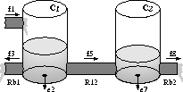
For example, consider the bi-tank system in Fig. 1. If
the left outflow blocks, ![]() , the level in both of the tanks starts
to rise. This abnormally high level may cause damage to the right outflow,
, the level in both of the tanks starts
to rise. This abnormally high level may cause damage to the right outflow,
![]() . However,
. However, ![]() causes the tank pressures to decrease
which masks the initial fault
causes the tank pressures to decrease
which masks the initial fault ![]() .
.
In real situations, desired measurement points are often inaccessible or the state of the art of sensor technology is such that sensors to measure desired variables are either inaccurate or very expensive, therefore, they are not used. Moreover, regulatory laws may require certain measurements to be made. Therefore, the set of measurements available for analysis may differ from the desired set, which makes it important to analyze which sets of faults can actually be discriminated. This is referred to as the diagnosability problem.
Early work by deKleer and Williams [3] used decision-theoretic methods for selecting the next best measurement in a sequential diagnosis framework. These ideas were further developed by Yu and Biswas [10] for steady state diagnosis of continuous systems. In other work, Chien, Doyle, and de Mello [2] developed four analysis methods for measurement selection: (i) sensitivity analysis measures which quantities have the greatest impact on the overall system state, (ii) cascading alarm analysis, which measures how alarms may cause other alarms to occur, (iii) potential damage analysis suggests which quantities in a system are likely to cause permanent damage, and (iv) teleological analysis ranks sensor placement according to the intended functionality of the system.
Based on a failure propagation graph, Misra et al. [5] define three metrics to evaluate diagnosability of complex dynamic systems: (i) detectability, the maximum time needed to detect a fault, (ii) predictability, the minimum time between a predicted fault and its actual occurrence, and (iii) distinguishability, the size of the set of hypothesized faults for a given time limit. In this paper we focus on the latter of these three criteria.
Our work on fault detection and analysis in complex, continuous dynamic systems exploits characteristics of transients in system behavior to identify abrupt faults in system components. These faults cause discontinuous changes in system parameters and move the system away from its nominal steady state. In time, a new steady state may be reached or the system may return to its original steady state. We first outline our approach to monitoring, prediction, and fault analysis. Next, we investigate measurement selection tasks in our diagnosis framework. Finally, we demonstrate the scalability of our approach by applying the measurement selection algorithms to a model of the secondary cooling system of a fast breeder reactor.